
Imagine you have a two group between-S study with N=30 in each group. You compute a two-sample t-test and the result is p = .09, not statistically significant with an effect size r = .17. Unbeknownst to you there is really no relationship between the IV and the DV. But, because you believe there is a relationship (you decided to run the study after all!), you think maybe adding five more subjects to each condition will help clarify things. So now you have N=35 in each group and you compute your t-test again. Now p = .04 with r = .21.
If you are reading this blog you might recognize what happened here as an instance of p-hacking. This particular form (testing periodically as you increase N) of p-hacking was one of the many data analytic flexibility issues exposed by Simmons, Nelson, and Simonshon (2011). But what are the real consequences of p-hacking? How often will p-hacking turn a null result into a positive result? What is the impact of p-hacking on effect size?
These were the kinds of questions that I had. So I wrote a little R function that simulates this type of p-hacking. The function – called phack – is designed to be flexible, although right now it only works for two-group between-S designs. The user is allowed to input and manipulate the following factors (argument name in parentheses):
- Initial Sample Size (initialN): The initial sample size (for each group) one had in mind when beginning the study (default = 30).
- Hack Rate (hackrate): The number of subjects to add to each group if the p-value is not statistically significant before testing again (default = 5).
- Population Means (grp1M, grp2M): The population means (Mu) for each group (default 0 for both).
- Population SDs (grp1SD, grp2SD): The population standard deviations (Sigmas) for each group (default = 1 for both).
- Maximum Sample Size (maxN): You weren’t really going to run the study forever right? This is the sample size (for each group) at which you will give up the endeavor and go run another study (default = 200).
- Type I Error Rate (alpha): The value (or lower) at which you will declare a result statistically significant (default = .05).
- Hypothesis Direction (alternative): Did your study have a directional hypothesis? Two-group studies often do (i.e., this group will have a higher mean than that group). You can choose from “greater” (Group 1 mean is higher), “less” (Group 2 mean is higher), or “two.sided” (any difference at all will work for me, thank you very much!). The default is “greater.”
- Display p-curve graph (graph)?: The function will output a figure displaying the p-curve for the results based on the initial study and the results for just those studies that (eventually) reached statistical significance (default = TRUE). More on this below.
- How many simulations do you want (sims). The number of times you want to simulate your p-hacking experiment.
To make this concrete, consider the following R code:
res <- phack(initialN=30, hackrate=5, grp1M=0, grp2M=0, grp1SD=1, grp2SD=1, maxN=200, alpha=.05, alternative="greater", graph=TRUE, sims=1000)
This says you have planned a two-group study with N=30 (initialN=30) in each group. You are going to compute your t-test on that initial sample. If that is not statistically significant you are going to add 5 more (hackrate=5) to each group and repeat that process until it is statistically significant or you reach 200 subjects in each group (maxN=200). You have set the population Ms to both be 0 (grp1M=0; grp2M=0) with SDs of 1 (grp1SD=1; grp2SD=1). You have set your nominal alpha level to .05 (alpha=.05), specified a direction hypothesis where group 1 should be higher than group 2 (alternative=“greater”), and asked for graphical output (graph=TRUE). Finally, you have requested to run this simulation 1000 times (sims=1000).
So what happens if we run this experiment?* So we can get the same thing, I have set the random seed in the code below.
source("http://rynesherman.com/phack.r") # read in the p-hack function
set.seed(3)
res <- phack(initialN=30, hackrate=5, grp1M=0, grp2M=0, grp1SD=1, grp2SD=1, maxN=200, alpha=.05, alternative="greater", graph=TRUE, sims=1000)
The following output appears in R:
Proportion of Original Samples Statistically Significant = 0.054
Proportion of Samples Statistically Significant After Hacking = 0.196
Probability of Stopping Before Reaching Significance = 0.805
Average Number of Hacks Before Significant/Stopping = 28.871
Average N Added Before Significant/Stopping = 144.355
Average Total N 174.355
Estimated r without hacking 0
Estimated r with hacking 0.03
Estimated r with hacking 0.19 (non-significant results not included)
The first line tells us how many (out of the 1000 simulations) of the originally planned (N=30 in each group) studies had a p-value that was .05 or less. Because there was no true effect (grp1M = grp2M) this at just about the nominal rate of .05. But what if we had used our p-hacking scheme (testing every 5 subjects per condition until significant or N=200)? That result is in the next line. It shows that just about 20% of the time we would have gotten a statistically significant result. So this type of hacking has inflated our Type I error rate from 5% to 20%. How often would we have given up (i.e., N=200) before reaching statistical significance? That is about 80% of the time. We also averaged 28.87 “hacks” before reaching significance/stopping, averaged having to add N=144 (per condition) before significance/stopping, and had an average total N of 174 (per condition) before significance/stopping.
What about effect sizes? Naturally the estimated effect size (r) was .00 if we just used our original N=30 in each group design. If we include the results of all 1000 completed simulations that effect size averages out to be r = .03. Most importantly, if we exclude those studies that never reached statistical significance, our average effect size r = .19.
This is pretty telling. But there is more. We also get this nice picture:
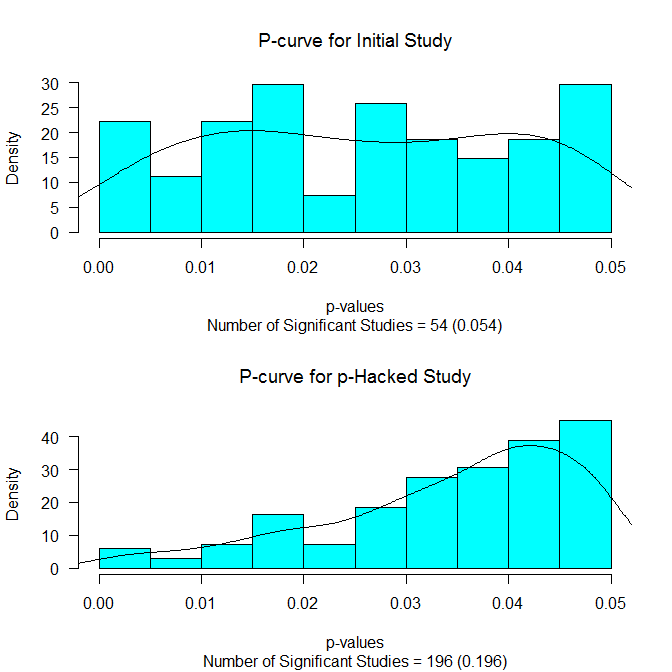
It shows the distribution of the p-values below .05 for the initial study (upper panel) and for those p-values below .05 for those reaching statistical significance. The p-curves (see Simonsohn, Nelson, & Simmons, 2013) are also drawn on. If there is really no effect, we should see a flat p-curve (as we do in the upper panel). And if there is no effect and p-hacking has occurred, we should see a p-curve that slopes up towards the critical value (as we do in the lower panel).
Finally, the function provides us with more detailed output that is summarized above. We can get a glimpse of this by running the following code:
head(res)
This generates the following output:
   Initial.p  Hackcount     Final.p  NAdded    Initial.r       Final.r
1 0.86410908         34  0.45176972     170  -0.14422580   0.006078565
2 0.28870264         34  0.56397332     170   0.07339944  -0.008077691
3 0.69915219         27  0.04164525     135  -0.06878039   0.095492249
4 0.84974744         34  0.30702946     170  -0.13594941   0.025289555
5 0.28048754         34  0.87849707     170   0.07656582  -0.058508736
6 0.07712726         34  0.58909693     170   0.18669338  -0.011296131
The object res contains the key results from each simulation including the p-value for the initial study (Initial.p), the number of times we had to hack (Hackcount), the p-value for the last study run (Final.p), the total N added to each condition (NAdded), the effect size r for the initial study (Initial.r), and the effect size r for the last study run (Final.r).
So what can we do with this? I see lots of possibilities and quite frankly I don’t have the time or energy to do them. Here are some quick ideas:
- What would happen if there were a true effect?
- What would happen if there were a true (but small) effect?
- What would happen if we checked for significance after each subject (hackrate=1)?
- What would happen if the maxN were lower?
- What would happen if the initial sample size was larger/smaller?
- What happens if we set the alpha = .10?
- What happens if we try various combinations of these things?
I’ll admit I have tried out a few of these ideas myself, but I haven’t really done anything systematic. I just thought other people might find this function interesting and fun to play with.
* By the way, all of these arguments are set to their default, so you can do the same thing by simply running res <- phack()
Update (10/11/2014) phackRM() is now available at http://rynesherman.com/phackRM.r to simulate p-hacking for dependent samples.
Pingback: P-Hacking True Effects
Pingback: A lesson from R-fortunes: all science is not good science. | Serfass Research
Thank you for writing and posting this helpful function!
If the t-test for the 1st wave reveals a statistically significant difference, can I use the size of this wave for the hackrate argument? In other words, what if a researcher is testing whether an effect “holds”–can s/he use your function?
Correction: not the 1st wave size as the hackrate argument.
Hi Nick,
I think I understand your question. If you have N=30 participants, get p < .05 and then subsequently add 10 more subjects, what happens then? It's a little tricky to handle with my function because we would need to know if you plan on adding 10 more subjects regardless of the results. If the plan all along was to add more subjects no matter what, then there is no worry about p-hacking. You can just report the final results. However, if there was never any plan to add more subjects until after the data were gathered, there would probably need to be some adjustment done. The proper adjustment might depend on what made you decide to collect more. This function assumes that thing that made you decide that was p > .05. But in your example case, it is just the opposite, p < .05. This makes me think something like sequential analysis may be useful: http://daniellakens.blogspot.com/2014/06/data-peeking-without-p-hacking.html
I hope that helps. :-/
I just wrote something like this the other day! I wish I’d found your first. 🙂