Tag Archives: R

Developing Short Measures of Broad Constructs: Issues of Reliability and Validity

Consider the following problem. I have a 4-item measure of a psychological construct. Let’s call it Extraversion. Here are the four items:

  • I like to go to parties
  • I am a talkative person
  • I see myself as a good leader
  • I like to take charge

It might be obvious to some, but the first two items and the last two items are more related to each other than the other combinations of items. In fact, we could say the first two items measure the “Sociability” aspect of Extraversion while the last two items measure the “Assertiveness” aspect of Extraversion.

Now let’s say I am in a real bind because, although I love my 4-item measure of Extraversion, in my next study I only have time for a 2-item measure. Which two items should I choose?

Let’s further say that I have collected a lot of data using our 4-item measure and know that the correlation matrix among the items looks like this:

Item 1 Item 2 Item 3 Item 4
Item 1 1.00 .80 .30 .30
Item 2 1.00 .30 .30
Item 3 1.00 .80
Item 4 1.00


So as noted above, the first two items and the last two items are highly correlated, but all items are at least moderately associated. So which two items should I choose?

The Case for High Internal Consistency

At some point, almost every psychology student is taught that reliability limits validity. That is, on average, the correlation between two constructs cannot exceed the square root of the product of their reliabilities. Or more simply, scales with higher reliability can achieve higher validity. The most frequently used method of estimating reliability is undoubtedly Cronbach’s alpha. Cronbach’s alpha is a measure of the internal consistency of a scale (assuming a single factor underlies the scale). Cronbach’s alpha is also an estimate of reliability under the special condition that the items making up the scale can be thought of as a random subset of the population of items that could make up the scale. With this in mind, the obvious choices are to go with either Items 1 and 2 or Items 3 and 4. Either of those combinations will certainly have higher internal consistency in our new study.

The Case for Content Coverage

However, if we select one of the high internal consistency options, we are sacrificing content coverage in our measure. Indeed, one could easily argue that our shorter measure is now either a measure of Sociability or Assertiveness, but not Extraversion. From a logical standpoint, if we want to cover our entire construct, we should choose those items that are the least correlated with each other (in this case that any of the following combinations: 1_3, 1_4, 2_3, or 2_4). Unfortunately, all of these choices are going to have lower internal consistencies. And as noted above, a low reliability will limit our validity. Or will it?

I’ve created an example in R to work through this hypothetical, but relatively realistic, problem. Let’s first begin by creating our population correlation matrix. We will then use that population correlation matrix to generate some random data to test out our different options. Of course, because we want to examine validity, we need some sort of criterion. So to our matrix from above, I’ve added a fifth variable – let’s call it popularity – and I’m assuming this variable correlates r = .10 with each of our items (i.e., has some small degree of validity).


library(mvtnorm)

mat <- matrix(c(1,.8,.3,.3,.1,

.8,1,.3,.3,.1,

.3,.3,1,.8,.1,

.3,.3,.8,1,.1,

.1,.1,.1,.1,1),

ncol=5, byrow=T)

set.seed(12345) # See we can get the same results

dat <- rmvnorm(n=10000, sigma=mat)

cor(dat[,1:4]) # Our sample correlation matrix for our key items

[,1] [,2] [,3] [,4]

[1,] 1.0 0.8 0.3 0.3

[2,] 0.8 1.0 0.3 0.3

[3,] 0.3 0.3 1.0 0.8

[4,] 0.3 0.3 0.8 1.0

As noted above, there are six possible combinations of items to form composites we could choose from: 1_2, 1_3, 1_4, 2_3, 2_4, and 3_4. One thing that might tip our decision about which to use is to first determine which combination of items correlates most closely with the scores we would get from our 4-item measure. The partwhole() function in the {multicon} package does this for us rapidly:


library(multicon)

partwhole(dat[,1:4], nitems=2)

The argument nitems=2 tells the function that we want to look at all of the possible 2-item combinations. The results look like this (note I’ve rounded them here):


1_2 1_3 1_4 2_3 2_4 3_4

Umatch 0.82 0.96 0.96 0.96 0.96 0.82

Fmatch 0.81 0.96 0.96 0.96 0.96 0.82

The top row (1_2, 1_3, etc.) identifies the combination of items that was used to form a composite. The next row (Umatch) are the partwhole correlations between the scores for that two-item composite, using unit weighting, and the total scores yielded by averaging all four items. The third row (Fmatch) contains the partwhole correlations between the scores for that two-item composite, using component scores, and the total scores yielded from a single principle component of all four items. The numbers are very similar across rows, but in this case we care more about Umatch because we intend on creating a unit-weighted composite with our new measure.

What should be obvious from this pattern of results is that the four combinations of items that select one item from each aspect (Sociability and Assertiveness) have much stronger partwhole correlations than either of the other two (more internally consistent) combinations.

What about internal consistency? We can get the internal consistency (alpha) for our four-item measure and for each possible combination of two items measures:


alpha.cov(cor(dat[,1:4]))

# For various combinations of 2 items

alpha.cov(cor(dat[,1:2]))

alpha.cov(cor(dat[,c(1,3)]))

alpha.cov(cor(dat[,c(1,4)]))

alpha.cov(cor(dat[,2:3]))

alpha.cov(cor(dat[,c(2,4)]))

alpha.cov(cor(dat[,3:4]))

The internal consistencies are .78 for the 4-item measure, .89 for the two Sociability items and .88 for the two Assertiveness items. Those are fairly high and fall into what many psychologists might call the “acceptable” range for reliability. The other four combinations do not fare so well with reliabilities of .46. Many people would consider these “unacceptably low.” So clearly, combinations 1_2 and 3_4 are the winners from an internal consistency standpoint.

But what about validity? Arguably, the entire point of the scientific enterprise is validity. Indeed, some might argue that the whole point of measurement is prediction. So how do our six combinations of 2-item scales do in terms of predicting our criterion?

We can use the scoreTest() function, available in the {multicon} package[1], to create our six composite scores.


myKeys <- list(OneTwo = c(1,2), OneThree = c(1,3), OneFour = c(1,4),

TwoThree = c(2,3), TwoFour = c(2,4), ThreeFour = c(3,4))

out <- scoreTest(data.frame(dat), myKeys, rel=TRUE)

out$rel # The same alphas as before with more information

describe(out$scores)

Note that scoreTest() has an option for calculating the alphas (and other metrics of internal consistency). You can check those for consistency with the above.

Now let’s correlate our six composites with the criterion. But beyond these validity coefficients, we might also want to look at the validities if we correct for attenuation. We can do the latter by simply dividing the observed correlations by the square root of their estimated reliabilities (internal consistencies).


ObsCors <- cor(out$scores, dat[,5])

DisCors <- ObsCors / sqrt(out$rel[,1])

# Which combination is best as predicting the criterion?

round(data.frame("r"=ObsCors, "rho"=DisCors),2)

r rho

OneTwo   0.10 0.11

OneThree 0.12 0.18

OneFour   0.13 0.19

TwoThree 0.12 0.17

TwoFour   0.12 0.18

ThreeFour 0.11 0.11

So how do our results look? First in terms of observed correlations (r), the constructs that used one item from Sociability and Assertiveness outperform the constructs that use only Sociability or Assertiveness items. The picture is even clearer when we look at the corrected correlations (rho). By virtue of their high internal consistencies, neither the pure Sociability nor the pure Assertiveness composites gain much when corrected for unreliability.

So it seems, in regards to our hypothetical case here, we should prefer any combination of items that uses one Sociability and one Assertiveness item when creating our new 2-item measure of Extraversion. This might seem counterintuitive to some. To others, this might seem obvious. And actually, Guilford (1954) showed this a long time ago in his equation 14.37:

GuilfordEq

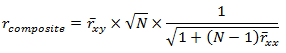
In this equation, rcomposite is the validity of a composite of N items, rxy is the average validity of each item in the composite, and rxx is the average inter-correlation of the items forming the composite. The simple R script below applies Guilford’s equation to our situation.


# Applying Guilford's Equation

AvgItemValidities <- rep(.1, 6)

NItems <- 2

AvgItemCors <- c(.8,.3,.3,.3,.3,.8)

&nbsp;

guilford <- function(rXY, N, rXX) {

return(rXY * sqrt(N) * 1 / sqrt(1 + (N - 1)*rXX))

}

round(guilford(AvgItemValidities, NItems, AvgItemCors),3)

[1] 0.105 0.124 0.124 0.124 0.124 0.105

And the results are almost dead-on with what our simulation shows. That is, holding the number of items and the average validity of the items constant, increased internal consistency decreases composite validity. I’m not sure how many people know this. And amongst those who do, it is not clear to me how many people appreciate this fact.

Finally, to those who think this seems obvious, let me throw one more wrinkle at you. In measurement contexts (i.e., scale development) confirmatory factor analysis (CFA) is a common practice. Many people, especially reviewers, hold CFA fit results in high esteem. That is, if the model shows poor fit, it is invalid. Now, with a two-item measure, we cannot conduct a CFA because we do not have enough degrees of freedom. However, if we conduct “mental CFAs” for each of our six possible composite measures, it is obvious that model 1_2 and model 3_4 will show much better fits (i.e., they will have smaller residuals) than any of the other models. We could actually demonstrate this if we extended our example to six items and attempted to make a shorter 3-item measure. Thus, I suspect that even though much of what I said above might seem obvious to some, I also suspect that many would miss the fact that a poor CFA fit does not necessarily mean that the construct(s) being measured have poor validity. In fact, it is very possible that constructs formed from better fitting CFAs have worse predictive validity than constructs from worse fitting CFAs.

[1] This function is only available in version >=1.5 of the{multicon} package released after 1/8/2015. If you have an older version, you may need to update.

Reference

Guilford, J. P. (1954). Psychometric Methods (2nd ed.). New York: McGraw-Hill.

Note: I am grateful to Tal Yarkoni for his feedback on a prior draft of this post.

(Mis)Interpreting Confidence Intervals

In a recent paper Hoekstra, Morey, Rouder, & Wagenmakers argued that confidence intervals are just as prone to misinterpretation as tradiational p-values (for a nice summary, see this blog post). They draw this conclusion based on responses to six questions from 442 bachelor students, 34 master students, and 120 researchers (PhD students and faculty). The six questions were of True / False format and are shown here (this is taken directly from their Appendix, please don’t sue me; if I am breaking the law I will remove this without hesitation):

Bubledorf

Hoekstra et al. note that all six statements are false and therefore the correct response to mark each as False. [1] The results were quite disturbing. The average number of statements marked True, across all three groups, was 3.51 (58.5%). Particularly disturbing is the fact that statement #3 was endorsed by 73%, 68%, and 86% of bachelor students, master students, and researchers respectively. Such a finding demonstrates that people often use confidence intervals simply to revert back to NHST (i.e., if the CI does not contain zero, reject the null).

However, it was questions #4 and #5 that caught my attention when reading this study. The reason they caught my attention is because my understanding of confidence intervals told me they are correct. However, the correct interpretation of a confidence interval, according to Hoekstra et al., is “If we were to repeat the experiment over and over, then 95% of the time the confidence intervals contain the true mean.” Now, if you are like me, you might be wondering, how is that different from a 95% probability that the true mean lies between the interval? Despite the risk of looking ignorant, I asked that very question on Twitter:

TwitterPic

Alexander Etz (@AlexanderEtz) provided an excellent answer to my question. His post is rather short, but I’ll summarize it here anyway: from a Frequentist framework (under which CIs fall), one cannot assign a probability to a single event, or in this case, a single CI. That is, the CI either contains μ (p = 1) or it does not (p = 0), from a Frequentist perspective.

Despite Alexander’s clear (and correct) explanation, I still reject it. I reject it on the grounds that it is practically useful to think of a single CI as having a 95% chance of containing μ. I’m not alone here. Geoff Cumming also thinks so. In his book (why haven’t you bought this book yet?) on p. 78 he provides two interpretations for confidence intervals that match my perspective. The first interpretation is “One from the Dance of CIs.” This interpretation fits precisely with Hoekstra et al.’s definition. If we repeated the experiment indefinitely we would approach an infinite number of CIs and 95% of those would contain μ. The second interpretation (“Interpret our Interval”) says the following:

It’s tempting to say that the probability is .95 that μ lies in our 95% CI. Some scholars permit such statements, while others regard them as wrong, misleading, and wicked. The trouble is that mention of probability suggests μ is a variable, rather than having a fixed value that we don’t know. Our interval either does or does not include μ, and so in a sense the probability is either 1 or 0. I believe it’s best to avoid the term “probability,” to discourage any misconception that μ is a variable. However, in my view it’s acceptable to say, “We are 95% confidence that our interval includes μ,” provided that we keep in the back of our minds that we’re referring to 95% of the intervals in the dance including μ, and 5% (the red ones) missing μ.

So in Cumming’s view, question #4 would still be False (because it misleads one to thinking that μ is a variable), but #5 would be True. Regardless, it seems clear that there is some debate about whether #4 and #5 are True or False. My personal belief is that it is okay to mark them both True. I’ve built a simple R example to demonstrate why.

# First, create 1000 datasets of N=100 each from a normal distribution.
set.seed(5)
sims <- 1000
datasets <- list()
for(i in 1:sims) {
  datasets[[i]] <- rnorm(100)
}

  # Now get the 95% confidence interval for each dataset.
out <- matrix(unlist(lapply(datasets, function(x) t.test(x)$conf.int)), ncol=2, byrow=T)
colnames(out) <- c("LL", "UL")
  # Count the number of confidence intervals containing Mu
res <- ifelse(out[,1] <= 0 & out[,2] >= 0, 1, 0)
sum(res) / sims
  # Thus, ~95% of our CIs contain Mu

This code creates 1000 datasets of N=100 by randomly drawing scores from a normal distribution with μ = 0 and σ = 1. It then computes a 95% confidence interval for the mean for each dataset. Lastly, it counts how many of those contain μ (0). In this case, it is just about 95%.[2] This is precisely the definition of a confidence interval provided by Hoekstra et al. If we repeat an experiment many times, 95% of our confidence intervals should contain μ. However, if we were just given one of those confidence intervals (say, at random) there would also be a 95% chance it contains μ. So if we think of our study, and its confidence interval, as one of many possible studies and intervals, we can be 95% confident that this particular interval contains the population value.

Moreover, this notion can be extended beyond a single experiment. That is, rather than thinking about repeating the same experiment many times, we can think of all of the different experiments (on different topics with different μs) we conduct and note that 95% of them will contain μ within the confidence interval, but 5% will not. Therefore, while I (think) I understand and appreciate why Hoekstra et al. consider the answers to #4 and #5 to be False, I disagree. I think that they are practically useful interpretations of a CI. If it violates all that is statistically holy and sacred, then damn me to statistical hell.

Despite this conclusion, I do not mean to undermine the research by Hoekstra et al. Indeed, my point has little bearing on the overall conclusion of their paper. Even if questions #4 and #5 were removed, the results are still incredibly disturbing and suggest that we need serious revisions to our statistical training.


[1] The last sentence of the instructions makes it clear that it is possible that all True and all False are possibilities. How many people actually believed that instruction is another question.

[2] Just for fun, I also calculated the proportion of times a given confidence interval contains the sample mean from a replication. The code you can run is below, but the answer is about 84.4%, which is close to Cummings’ (p. 128) CI Interpretation 6 “Prediction Interval for a Replication Mean” of 83%.

  # Now get the sample Means
Ms <- unlist(lapply(datasets, mean))
    # For each confidence interval, determine how many other sample means it captured
reptest <- sapply(Ms, function(x) ifelse(out[,1] <= x & out[,2] >= x, 1, 0))
      # Remove the diagonal to avoid double-counting
diag(reptest) <- NA
      # Now summarize it:
mean(colMeans(reptest, na.rm=T)) # So ~ 84.4% chance of a replication falling within the 95% CI


phack: An R Function for Examining the Effects of p-hacking

Imagine you have a two group between-S study with N=30 in each group. You compute a two-sample t-test and the result is p = .09, not statistically significant with an effect size r = .17. Unbeknownst to you there is really no relationship between the IV and the DV. But, because you believe there is a relationship (you decided to run the study after all!), you think maybe adding five more subjects to each condition will help clarify things. So now you have N=35 in each group and you compute your t-test again. Now p = .04 with r = .21.

If you are reading this blog you might recognize what happened here as an instance of p-hacking. This particular form (testing periodically as you increase N) of p-hacking was one of the many data analytic flexibility issues exposed by Simmons, Nelson, and Simonshon (2011). But what are the real consequences of p-hacking? How often will p-hacking turn a null result into a positive result? What is the impact of p-hacking on effect size?

These were the kinds of questions that I had. So I wrote a little R function that simulates this type of p-hacking. The function – called phack – is designed to be flexible, although right now it only works for two-group between-S designs. The user is allowed to input and manipulate the following factors (argument name in parentheses):

  • Initial Sample Size (initialN): The initial sample size (for each group) one had in mind when beginning the study (default = 30).
  • Hack Rate (hackrate): The number of subjects to add to each group if the p-value is not statistically significant before testing again (default = 5).
  • Population Means (grp1M, grp2M): The population means (Mu) for each group (default 0 for both).
  • Population SDs (grp1SD, grp2SD): The population standard deviations (Sigmas) for each group (default = 1 for both).
  • Maximum Sample Size (maxN): You weren’t really going to run the study forever right? This is the sample size (for each group) at which you will give up the endeavor and go run another study (default = 200).
  • Type I Error Rate (alpha): The value (or lower) at which you will declare a result statistically significant (default = .05).
  • Hypothesis Direction (alternative): Did your study have a directional hypothesis? Two-group studies often do (i.e., this group will have a higher mean than that group). You can choose from “greater” (Group 1 mean is higher), “less” (Group 2 mean is higher), or “two.sided” (any difference at all will work for me, thank you very much!). The default is “greater.”
  • Display p-curve graph (graph)?: The function will output a figure displaying the p-curve for the results based on the initial study and the results for just those studies that (eventually) reached statistical significance (default = TRUE). More on this below.
  • How many simulations do you want (sims). The number of times you want to simulate your p-hacking experiment.

To make this concrete, consider the following R code:

res <- phack(initialN=30, hackrate=5, grp1M=0, grp2M=0, grp1SD=1, grp2SD=1, maxN=200, alpha=.05, alternative="greater", graph=TRUE, sims=1000)

This says you have planned a two-group study with N=30 (initialN=30) in each group. You are going to compute your t-test on that initial sample. If that is not statistically significant you are going to add 5 more (hackrate=5) to each group and repeat that process until it is statistically significant or you reach 200 subjects in each group (maxN=200). You have set the population Ms to both be 0 (grp1M=0; grp2M=0) with SDs of 1 (grp1SD=1; grp2SD=1). You have set your nominal alpha level to .05 (alpha=.05), specified a direction hypothesis where group 1 should be higher than group 2 (alternative=“greater”), and asked for graphical output (graph=TRUE). Finally, you have requested to run this simulation 1000 times (sims=1000).

So what happens if we run this experiment?* So we can get the same thing, I have set the random seed in the code below.

source("http://rynesherman.com/phack.r") # read in the p-hack function
set.seed(3)
res <- phack(initialN=30, hackrate=5, grp1M=0, grp2M=0, grp1SD=1, grp2SD=1, maxN=200, alpha=.05, alternative="greater", graph=TRUE, sims=1000)

The following output appears in R:

Proportion of Original Samples Statistically Significant = 0.054
Proportion of Samples Statistically Significant After Hacking = 0.196
Probability of Stopping Before Reaching Significance = 0.805
Average Number of Hacks Before Significant/Stopping = 28.871
Average N Added Before Significant/Stopping = 144.355
Average Total N 174.355
Estimated r without hacking 0
Estimated r with hacking 0.03
Estimated r with hacking 0.19 (non-significant results not included)

The first line tells us how many (out of the 1000 simulations) of the originally planned (N=30 in each group) studies had a p-value that was .05 or less. Because there was no true effect (grp1M = grp2M) this at just about the nominal rate of .05. But what if we had used our p-hacking scheme (testing every 5 subjects per condition until significant or N=200)? That result is in the next line. It shows that just about 20% of the time we would have gotten a statistically significant result. So this type of hacking has inflated our Type I error rate from 5% to 20%. How often would we have given up (i.e., N=200) before reaching statistical significance? That is about 80% of the time. We also averaged 28.87 “hacks” before reaching significance/stopping, averaged having to add N=144 (per condition) before significance/stopping, and had an average total N of 174 (per condition) before significance/stopping.

What about effect sizes? Naturally the estimated effect size (r) was .00 if we just used our original N=30 in each group design. If we include the results of all 1000 completed simulations that effect size averages out to be r = .03. Most importantly, if we exclude those studies that never reached statistical significance, our average effect size r = .19.

This is pretty telling. But there is more. We also get this nice picture:

phackPic

It shows the distribution of the p-values below .05 for the initial study (upper panel) and for those p-values below .05 for those reaching statistical significance. The p-curves (see Simonsohn, Nelson, & Simmons, 2013) are also drawn on. If there is really no effect, we should see a flat p-curve (as we do in the upper panel). And if there is no effect and p-hacking has occurred, we should see a p-curve that slopes up towards the critical value (as we do in the lower panel).

Finally, the function provides us with more detailed output that is summarized above. We can get a glimpse of this by running the following code:

head(res)

This generates the following output:

   Initial.p  Hackcount     Final.p  NAdded    Initial.r       Final.r
1 0.86410908         34  0.45176972     170  -0.14422580   0.006078565
2 0.28870264         34  0.56397332     170   0.07339944  -0.008077691
3 0.69915219         27  0.04164525     135  -0.06878039   0.095492249
4 0.84974744         34  0.30702946     170  -0.13594941   0.025289555
5 0.28048754         34  0.87849707     170   0.07656582  -0.058508736
6 0.07712726         34  0.58909693     170   0.18669338  -0.011296131

The object res contains the key results from each simulation including the p-value for the initial study (Initial.p), the number of times we had to hack (Hackcount), the p-value for the last study run (Final.p), the total N added to each condition (NAdded), the effect size r for the initial study (Initial.r), and the effect size r for the last study run (Final.r).

So what can we do with this? I see lots of possibilities and quite frankly I don’t have the time or energy to do them. Here are some quick ideas:

  • What would happen if there were a true effect?
  • What would happen if there were a true (but small) effect?
  • What would happen if we checked for significance after each subject (hackrate=1)?
  • What would happen if the maxN were lower?
  • What would happen if the initial sample size was larger/smaller?
  • What happens if we set the alpha = .10?
  • What happens if we try various combinations of these things?

I’ll admit I have tried out a few of these ideas myself, but I haven’t really done anything systematic. I just thought other people might find this function interesting and fun to play with.

* By the way, all of these arguments are set to their default, so you can do the same thing by simply running res <- phack()


Update (10/11/2014) phackRM() is now available at http://rynesherman.com/phackRM.r to simulate p-hacking for dependent samples.