Tag Archives: Statistics

(Mis)Interpreting Confidence Intervals

In a recent paper Hoekstra, Morey, Rouder, & Wagenmakers argued that confidence intervals are just as prone to misinterpretation as tradiational p-values (for a nice summary, see this blog post). They draw this conclusion based on responses to six questions from 442 bachelor students, 34 master students, and 120 researchers (PhD students and faculty). The six questions were of True / False format and are shown here (this is taken directly from their Appendix, please don’t sue me; if I am breaking the law I will remove this without hesitation):

Bubledorf

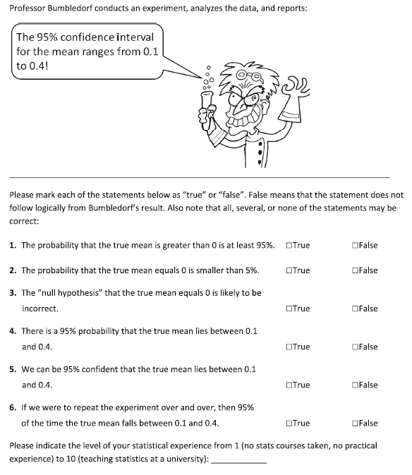
Hoekstra et al. note that all six statements are false and therefore the correct response to mark each as False. [1] The results were quite disturbing. The average number of statements marked True, across all three groups, was 3.51 (58.5%). Particularly disturbing is the fact that statement #3 was endorsed by 73%, 68%, and 86% of bachelor students, master students, and researchers respectively. Such a finding demonstrates that people often use confidence intervals simply to revert back to NHST (i.e., if the CI does not contain zero, reject the null).

However, it was questions #4 and #5 that caught my attention when reading this study. The reason they caught my attention is because my understanding of confidence intervals told me they are correct. However, the correct interpretation of a confidence interval, according to Hoekstra et al., is “If we were to repeat the experiment over and over, then 95% of the time the confidence intervals contain the true mean.” Now, if you are like me, you might be wondering, how is that different from a 95% probability that the true mean lies between the interval? Despite the risk of looking ignorant, I asked that very question on Twitter:

TwitterPic

Alexander Etz (@AlexanderEtz) provided an excellent answer to my question. His post is rather short, but I’ll summarize it here anyway: from a Frequentist framework (under which CIs fall), one cannot assign a probability to a single event, or in this case, a single CI. That is, the CI either contains μ (p = 1) or it does not (p = 0), from a Frequentist perspective.

Despite Alexander’s clear (and correct) explanation, I still reject it. I reject it on the grounds that it is practically useful to think of a single CI as having a 95% chance of containing μ. I’m not alone here. Geoff Cumming also thinks so. In his book (why haven’t you bought this book yet?) on p. 78 he provides two interpretations for confidence intervals that match my perspective. The first interpretation is “One from the Dance of CIs.” This interpretation fits precisely with Hoekstra et al.’s definition. If we repeated the experiment indefinitely we would approach an infinite number of CIs and 95% of those would contain μ. The second interpretation (“Interpret our Interval”) says the following:

It’s tempting to say that the probability is .95 that μ lies in our 95% CI. Some scholars permit such statements, while others regard them as wrong, misleading, and wicked. The trouble is that mention of probability suggests μ is a variable, rather than having a fixed value that we don’t know. Our interval either does or does not include μ, and so in a sense the probability is either 1 or 0. I believe it’s best to avoid the term “probability,” to discourage any misconception that μ is a variable. However, in my view it’s acceptable to say, “We are 95% confidence that our interval includes μ,” provided that we keep in the back of our minds that we’re referring to 95% of the intervals in the dance including μ, and 5% (the red ones) missing μ.

So in Cumming’s view, question #4 would still be False (because it misleads one to thinking that μ is a variable), but #5 would be True. Regardless, it seems clear that there is some debate about whether #4 and #5 are True or False. My personal belief is that it is okay to mark them both True. I’ve built a simple R example to demonstrate why.

# First, create 1000 datasets of N=100 each from a normal distribution.
set.seed(5)
sims <- 1000
datasets <- list()
for(i in 1:sims) {
  datasets[[i]] <- rnorm(100)
}

  # Now get the 95% confidence interval for each dataset.
out <- matrix(unlist(lapply(datasets, function(x) t.test(x)$conf.int)), ncol=2, byrow=T)
colnames(out) <- c("LL", "UL")
  # Count the number of confidence intervals containing Mu
res <- ifelse(out[,1] <= 0 & out[,2] >= 0, 1, 0)
sum(res) / sims
  # Thus, ~95% of our CIs contain Mu

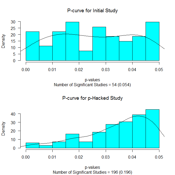
This code creates 1000 datasets of N=100 by randomly drawing scores from a normal distribution with μ = 0 and σ = 1. It then computes a 95% confidence interval for the mean for each dataset. Lastly, it counts how many of those contain μ (0). In this case, it is just about 95%.[2] This is precisely the definition of a confidence interval provided by Hoekstra et al. If we repeat an experiment many times, 95% of our confidence intervals should contain μ. However, if we were just given one of those confidence intervals (say, at random) there would also be a 95% chance it contains μ. So if we think of our study, and its confidence interval, as one of many possible studies and intervals, we can be 95% confident that this particular interval contains the population value.

Moreover, this notion can be extended beyond a single experiment. That is, rather than thinking about repeating the same experiment many times, we can think of all of the different experiments (on different topics with different μs) we conduct and note that 95% of them will contain μ within the confidence interval, but 5% will not. Therefore, while I (think) I understand and appreciate why Hoekstra et al. consider the answers to #4 and #5 to be False, I disagree. I think that they are practically useful interpretations of a CI. If it violates all that is statistically holy and sacred, then damn me to statistical hell.

Despite this conclusion, I do not mean to undermine the research by Hoekstra et al. Indeed, my point has little bearing on the overall conclusion of their paper. Even if questions #4 and #5 were removed, the results are still incredibly disturbing and suggest that we need serious revisions to our statistical training.


[1] The last sentence of the instructions makes it clear that it is possible that all True and all False are possibilities. How many people actually believed that instruction is another question.

[2] Just for fun, I also calculated the proportion of times a given confidence interval contains the sample mean from a replication. The code you can run is below, but the answer is about 84.4%, which is close to Cummings’ (p. 128) CI Interpretation 6 “Prediction Interval for a Replication Mean” of 83%.

  # Now get the sample Means
Ms <- unlist(lapply(datasets, mean))
    # For each confidence interval, determine how many other sample means it captured
reptest <- sapply(Ms, function(x) ifelse(out[,1] <= x & out[,2] >= x, 1, 0))
      # Remove the diagonal to avoid double-counting
diag(reptest) <- NA
      # Now summarize it:
mean(colMeans(reptest, na.rm=T)) # So ~ 84.4% chance of a replication falling within the 95% CI


When Are Direct Replications Necessary?

We are told that replication is the heart of all sciences. As such, psychology has recently seen numerous calls for direct replication. Sanjay Srivastava says that replication provides an opportunity to falsify an idea (an important concept in science, but rarely done in psychology). Brian Nosek and Jeffrey Spies suggest that replication would help identify “manufactured effects” rapidly. And Brent Roberts proposed a three step process, the last of which is a direct replication of any unique study reported in the package of studies.

Not everyone thinks that direct replications are useful though. Andrew Wilson has argued that replication will not save psychology and better theories are needed. Jason Mitchell has gone so far as to say that failed replications offer nothing to science as they are largely the result of practical mistakes on the part of the experimenters. So are direct replications necessary? My answer is a definitive: sometimes.

Let’s start by considering what I gather to be some of the main arguments for direct replications.

  • You might have screwed up the first study. This is one of the reasons Brent Roberts has proposed direct replications (see his response to my comment). Interestingly, this is the other side of the argument posed by Mitchell. That is, you could have typos in your measures, left questions off the survey, the coffee maker could have interfered with the EEG readings,[1] or the data could have been mishandled.
  • Direct replications, when combined with meta-analysis, yield more precise effect size estimates. What is better than one study with N=50? How about two studies with N=50 in each! Perspectives on Psychological Science is now accepting registered replication reports and one of the motivating principles is that “Direct replications are necessary to estimate the true size of an effect.” Likewise, Sean Mackinnon says “It is only through repeated experiments that we are able to center on an accurate estimate of the effect size.”
  • Direct replications can improve generalizability. All other things being equal, we would like our results to generalize to the largest group of people possible. If a study yields the expected results only when conducted on University of Michigan undergrads, we would not be so impressed. Direct replications by different investigators, in different locations, sampling from different sub-populations can offer critical information about generalizability.

But there are problems with these arguments:

  • You might have screwed up the first study. Yes, there may have been methodological problems and artifacts in the first study. But how is running a direct replication supposed to fix this problem?

My guess is that most modern labs gather data in a similar fashion to the way we gather data in my lab. One of my (super smart) graduate students logs into our survey software (we use Qualtrics) and types the survey in there, choosing the scale points, entering anchors, etc. We go through the survey ourselves checking for errors. Then we have Research Assistants do the same. Then we gather say N=5 data points (these data points are usually from members of the research team) and download the data to make sure we understand how the software is storing and returning the values we gave it. Then we run the study. Now, when it comes time to do another study do we start all over again? No. We simply click “copy survey” and the software makes a copy of the same survey we already used for another study. We can do that with lots of different surveys to the point that we almost never have to enter a survey by hand again.

Now these are not direct replications we are running. These are new studies using the same measures. But if we were running a direct replication, how would the process be different? It would be even worse because we wouldn’t even create anything new. We would just have new participants complete the same Qualtrics survey we created before noting which participants were new. So if we screwed up the measures the first time, they are still screwed up now.

Is this a new-age internet survey problem? I doubt it. When I was an undergraduate running experiments we essentially did the same thing only with paper copies. So if the anchor was off the first time someone created the survey (and no one noticed it), it was going to be off on every copy of that survey. And if we were running a direct replication, we wouldn’t start from scratch. We would just print out another copy of the same flawed survey.

Here is the good news though. With Open Science everyone can see what measures I used and how I screwed them up. Further, with open data everyone can see how the data were (mis)handled and if coffee makers created implausible outliers. Moreover, with scripted statistical analysis languages like R everyone can reproduce my results and see exactly where I screwed up the analysis (you can’t do that with point-and-click SPSS!).

Direct replications are not the solution to the problem of methodological/statistical flaws in the first study; Open Science is.

  • Direct replications, when combined with meta-analysis, yield more precise effect size estimates. This is absolutely 100% correct. It is also absolutely 100% unnecessary.

Consider three scenarios: (a) one study with n=20, (b) one study with n=400, (c) 20 studies with n=20 in each that are meta-analytically combined. Which of these will yield the most precise effect size estimate? Obviously it isn’t (a), but what about between (b) and (c)? This was precisely the topic of a post by Felix Schönbrodt. In it, Felix showed empirically that the precision of (b) and (c) are identical. While his post has great insights about precision, the empirical demonstration was (sorry Felix!) a bit useless. The mathematics of meta-analysis are some of the simplest in psychology and it is trivial to show that the standard error of an effect size based on N=400 is the same as one based on…errr, N=400.

So to put this bluntly, if we are interested in more precise effect sizes (and I think we should be), we don’t need direct replications. We need larger initial studies. Indeed, Schönbrodt and Perugini (2013) suggested that stable effect size estimates result when N=250.[2] If editors and reviewers considered sample size a more important criterion for publication there would be (a) fewer Type I errors in the literature, and (b) more precise effect size estimates (i.e., less over-estimated effect sizes due to publication bias). To underscore this point, consider the recent Facebook experiment that received much attention. The study had a total sample of N=689,003. On the scale of r the effect size estimates have a margin of error of ± .002. In one blog post about the study someone commented that the worst part is that because Facebook is so dominant in the SNS market that no one else will be able to replicate it to see if the effect really exists.[3] Seriously?!? Sorry. This study does not need to be directly replicated. The effect size estimates are pretty precise.

  • Direct replications can improve generalizability. YES! Direct replications are incredibly useful for improving generalizability.

The final argument for direct replications is to improve generalizability. This is the only reason that anyone should[4] call for direct replications. If I run a study on undergraduate students in south Florida (even with a large sample), you should in fact wonder if these results generalize to working adults in south Florida and to people from places all over the world. We probably have intuitions about which studies are likely to generalize and which ones aren’t, so we might rely on those to determine which studies are in most need of replication (for generalization purposes!). Or we might focus on trying to replicate studies that, if they are generalizable, would have the most practical and theoretical impact. I’d also suggest that we should periodically try to replicate important studies conducted some time ago (e.g., 20 years or more) just to be sure that the results generalize to modern people.

So to summarize, if we conduct good research in the first place, then we should[5] only need direct replications for generalizability purposes. If we find an error in a previously conducted study, then we should fix it. If that means running a new study with the error fixed, fine. But that isn’t a replication. It is a different (unflawed) study. And if we have good studies to begin with, we don’t need meta-analyses to provide more precise effect size estimates; we will already have them.

So, what constitutes a good study? We all probably have our own ideas, but I will provide my own personal criteria for study quality in another blog post.


[1] I have no idea if coffee makers can interfere with EEG machines. I don’t drink coffee.

[2] I think N=200 is a better number, but that is the subject of another blog post to come in the future (and also Simine Vazire’s suggestion!).

[3] I wish I had recorded the post and comment, but I didn’t. You’ll just have to take my word that it existed and I read it.

[4] I really want to emphasize should here because this is my fantasy-land where researchers actually care about precisely measuring natural relationships. If actions speak louder than words, we know that much research in psychology has little interest in precisely measuring natural relationships.

[5] See footnote 4. Please also note that I am only referring to direct replications here, not conceptual replications or extensions. Indeed, conceptual replications and extensions are crucial ways of demonstrating generalizability.

phack: An R Function for Examining the Effects of p-hacking

Imagine you have a two group between-S study with N=30 in each group. You compute a two-sample t-test and the result is p = .09, not statistically significant with an effect size r = .17. Unbeknownst to you there is really no relationship between the IV and the DV. But, because you believe there is a relationship (you decided to run the study after all!), you think maybe adding five more subjects to each condition will help clarify things. So now you have N=35 in each group and you compute your t-test again. Now p = .04 with r = .21.

If you are reading this blog you might recognize what happened here as an instance of p-hacking. This particular form (testing periodically as you increase N) of p-hacking was one of the many data analytic flexibility issues exposed by Simmons, Nelson, and Simonshon (2011). But what are the real consequences of p-hacking? How often will p-hacking turn a null result into a positive result? What is the impact of p-hacking on effect size?

These were the kinds of questions that I had. So I wrote a little R function that simulates this type of p-hacking. The function – called phack – is designed to be flexible, although right now it only works for two-group between-S designs. The user is allowed to input and manipulate the following factors (argument name in parentheses):

  • Initial Sample Size (initialN): The initial sample size (for each group) one had in mind when beginning the study (default = 30).
  • Hack Rate (hackrate): The number of subjects to add to each group if the p-value is not statistically significant before testing again (default = 5).
  • Population Means (grp1M, grp2M): The population means (Mu) for each group (default 0 for both).
  • Population SDs (grp1SD, grp2SD): The population standard deviations (Sigmas) for each group (default = 1 for both).
  • Maximum Sample Size (maxN): You weren’t really going to run the study forever right? This is the sample size (for each group) at which you will give up the endeavor and go run another study (default = 200).
  • Type I Error Rate (alpha): The value (or lower) at which you will declare a result statistically significant (default = .05).
  • Hypothesis Direction (alternative): Did your study have a directional hypothesis? Two-group studies often do (i.e., this group will have a higher mean than that group). You can choose from “greater” (Group 1 mean is higher), “less” (Group 2 mean is higher), or “two.sided” (any difference at all will work for me, thank you very much!). The default is “greater.”
  • Display p-curve graph (graph)?: The function will output a figure displaying the p-curve for the results based on the initial study and the results for just those studies that (eventually) reached statistical significance (default = TRUE). More on this below.
  • How many simulations do you want (sims). The number of times you want to simulate your p-hacking experiment.

To make this concrete, consider the following R code:

res <- phack(initialN=30, hackrate=5, grp1M=0, grp2M=0, grp1SD=1, grp2SD=1, maxN=200, alpha=.05, alternative="greater", graph=TRUE, sims=1000)

This says you have planned a two-group study with N=30 (initialN=30) in each group. You are going to compute your t-test on that initial sample. If that is not statistically significant you are going to add 5 more (hackrate=5) to each group and repeat that process until it is statistically significant or you reach 200 subjects in each group (maxN=200). You have set the population Ms to both be 0 (grp1M=0; grp2M=0) with SDs of 1 (grp1SD=1; grp2SD=1). You have set your nominal alpha level to .05 (alpha=.05), specified a direction hypothesis where group 1 should be higher than group 2 (alternative=“greater”), and asked for graphical output (graph=TRUE). Finally, you have requested to run this simulation 1000 times (sims=1000).

So what happens if we run this experiment?* So we can get the same thing, I have set the random seed in the code below.

source("http://rynesherman.com/phack.r") # read in the p-hack function
set.seed(3)
res <- phack(initialN=30, hackrate=5, grp1M=0, grp2M=0, grp1SD=1, grp2SD=1, maxN=200, alpha=.05, alternative="greater", graph=TRUE, sims=1000)

The following output appears in R:

Proportion of Original Samples Statistically Significant = 0.054
Proportion of Samples Statistically Significant After Hacking = 0.196
Probability of Stopping Before Reaching Significance = 0.805
Average Number of Hacks Before Significant/Stopping = 28.871
Average N Added Before Significant/Stopping = 144.355
Average Total N 174.355
Estimated r without hacking 0
Estimated r with hacking 0.03
Estimated r with hacking 0.19 (non-significant results not included)

The first line tells us how many (out of the 1000 simulations) of the originally planned (N=30 in each group) studies had a p-value that was .05 or less. Because there was no true effect (grp1M = grp2M) this at just about the nominal rate of .05. But what if we had used our p-hacking scheme (testing every 5 subjects per condition until significant or N=200)? That result is in the next line. It shows that just about 20% of the time we would have gotten a statistically significant result. So this type of hacking has inflated our Type I error rate from 5% to 20%. How often would we have given up (i.e., N=200) before reaching statistical significance? That is about 80% of the time. We also averaged 28.87 “hacks” before reaching significance/stopping, averaged having to add N=144 (per condition) before significance/stopping, and had an average total N of 174 (per condition) before significance/stopping.

What about effect sizes? Naturally the estimated effect size (r) was .00 if we just used our original N=30 in each group design. If we include the results of all 1000 completed simulations that effect size averages out to be r = .03. Most importantly, if we exclude those studies that never reached statistical significance, our average effect size r = .19.

This is pretty telling. But there is more. We also get this nice picture:

phackPic

It shows the distribution of the p-values below .05 for the initial study (upper panel) and for those p-values below .05 for those reaching statistical significance. The p-curves (see Simonsohn, Nelson, & Simmons, 2013) are also drawn on. If there is really no effect, we should see a flat p-curve (as we do in the upper panel). And if there is no effect and p-hacking has occurred, we should see a p-curve that slopes up towards the critical value (as we do in the lower panel).

Finally, the function provides us with more detailed output that is summarized above. We can get a glimpse of this by running the following code:

head(res)

This generates the following output:

   Initial.p  Hackcount     Final.p  NAdded    Initial.r       Final.r
1 0.86410908         34  0.45176972     170  -0.14422580   0.006078565
2 0.28870264         34  0.56397332     170   0.07339944  -0.008077691
3 0.69915219         27  0.04164525     135  -0.06878039   0.095492249
4 0.84974744         34  0.30702946     170  -0.13594941   0.025289555
5 0.28048754         34  0.87849707     170   0.07656582  -0.058508736
6 0.07712726         34  0.58909693     170   0.18669338  -0.011296131

The object res contains the key results from each simulation including the p-value for the initial study (Initial.p), the number of times we had to hack (Hackcount), the p-value for the last study run (Final.p), the total N added to each condition (NAdded), the effect size r for the initial study (Initial.r), and the effect size r for the last study run (Final.r).

So what can we do with this? I see lots of possibilities and quite frankly I don’t have the time or energy to do them. Here are some quick ideas:

  • What would happen if there were a true effect?
  • What would happen if there were a true (but small) effect?
  • What would happen if we checked for significance after each subject (hackrate=1)?
  • What would happen if the maxN were lower?
  • What would happen if the initial sample size was larger/smaller?
  • What happens if we set the alpha = .10?
  • What happens if we try various combinations of these things?

I’ll admit I have tried out a few of these ideas myself, but I haven’t really done anything systematic. I just thought other people might find this function interesting and fun to play with.

* By the way, all of these arguments are set to their default, so you can do the same thing by simply running res <- phack()


Update (10/11/2014) phackRM() is now available at http://rynesherman.com/phackRM.r to simulate p-hacking for dependent samples.