
In a recent paper Hoekstra, Morey, Rouder, & Wagenmakers argued that confidence intervals are just as prone to misinterpretation as tradiational p-values (for a nice summary, see this blog post). They draw this conclusion based on responses to six questions from 442 bachelor students, 34 master students, and 120 researchers (PhD students and faculty). The six questions were of True / False format and are shown here (this is taken directly from their Appendix, please don’t sue me; if I am breaking the law I will remove this without hesitation):
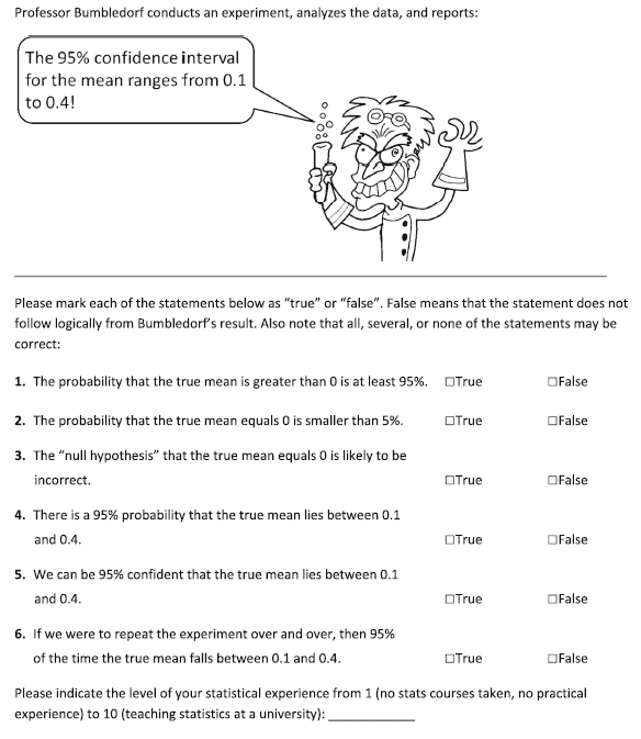
Hoekstra et al. note that all six statements are false and therefore the correct response to mark each as False. [1] The results were quite disturbing. The average number of statements marked True, across all three groups, was 3.51 (58.5%). Particularly disturbing is the fact that statement #3 was endorsed by 73%, 68%, and 86% of bachelor students, master students, and researchers respectively. Such a finding demonstrates that people often use confidence intervals simply to revert back to NHST (i.e., if the CI does not contain zero, reject the null).
However, it was questions #4 and #5 that caught my attention when reading this study. The reason they caught my attention is because my understanding of confidence intervals told me they are correct. However, the correct interpretation of a confidence interval, according to Hoekstra et al., is “If we were to repeat the experiment over and over, then 95% of the time the confidence intervals contain the true mean.” Now, if you are like me, you might be wondering, how is that different from a 95% probability that the true mean lies between the interval? Despite the risk of looking ignorant, I asked that very question on Twitter:

Alexander Etz (@AlexanderEtz) provided an excellent answer to my question. His post is rather short, but I’ll summarize it here anyway: from a Frequentist framework (under which CIs fall), one cannot assign a probability to a single event, or in this case, a single CI. That is, the CI either contains μ (p = 1) or it does not (p = 0), from a Frequentist perspective.
Despite Alexander’s clear (and correct) explanation, I still reject it. I reject it on the grounds that it is practically useful to think of a single CI as having a 95% chance of containing μ. I’m not alone here. Geoff Cumming also thinks so. In his book (why haven’t you bought this book yet?) on p. 78 he provides two interpretations for confidence intervals that match my perspective. The first interpretation is “One from the Dance of CIs.” This interpretation fits precisely with Hoekstra et al.’s definition. If we repeated the experiment indefinitely we would approach an infinite number of CIs and 95% of those would contain μ. The second interpretation (“Interpret our Interval”) says the following:
It’s tempting to say that the probability is .95 that μ lies in our 95% CI. Some scholars permit such statements, while others regard them as wrong, misleading, and wicked. The trouble is that mention of probability suggests μ is a variable, rather than having a fixed value that we don’t know. Our interval either does or does not include μ, and so in a sense the probability is either 1 or 0. I believe it’s best to avoid the term “probability,” to discourage any misconception that μ is a variable. However, in my view it’s acceptable to say, “We are 95% confidence that our interval includes μ,” provided that we keep in the back of our minds that we’re referring to 95% of the intervals in the dance including μ, and 5% (the red ones) missing μ.
So in Cumming’s view, question #4 would still be False (because it misleads one to thinking that μ is a variable), but #5 would be True. Regardless, it seems clear that there is some debate about whether #4 and #5 are True or False. My personal belief is that it is okay to mark them both True. I’ve built a simple R example to demonstrate why.
# First, create 1000 datasets of N=100 each from a normal distribution.
set.seed(5)
sims <- 1000
datasets <- list()
for(i in 1:sims) {
  datasets[[i]] <- rnorm(100)
}

  # Now get the 95% confidence interval for each dataset.
out <- matrix(unlist(lapply(datasets, function(x) t.test(x)$conf.int)), ncol=2, byrow=T)
colnames(out) <- c("LL", "UL")
  # Count the number of confidence intervals containing Mu
res <- ifelse(out[,1] <= 0 & out[,2] >= 0, 1, 0)
sum(res) / sims
  # Thus, ~95% of our CIs contain Mu
This code creates 1000 datasets of N=100 by randomly drawing scores from a normal distribution with μ = 0 and σ = 1. It then computes a 95% confidence interval for the mean for each dataset. Lastly, it counts how many of those contain μ (0). In this case, it is just about 95%.[2] This is precisely the definition of a confidence interval provided by Hoekstra et al. If we repeat an experiment many times, 95% of our confidence intervals should contain μ. However, if we were just given one of those confidence intervals (say, at random) there would also be a 95% chance it contains μ. So if we think of our study, and its confidence interval, as one of many possible studies and intervals, we can be 95% confident that this particular interval contains the population value.
Moreover, this notion can be extended beyond a single experiment. That is, rather than thinking about repeating the same experiment many times, we can think of all of the different experiments (on different topics with different μs) we conduct and note that 95% of them will contain μ within the confidence interval, but 5% will not. Therefore, while I (think) I understand and appreciate why Hoekstra et al. consider the answers to #4 and #5 to be False, I disagree. I think that they are practically useful interpretations of a CI. If it violates all that is statistically holy and sacred, then damn me to statistical hell.
Despite this conclusion, I do not mean to undermine the research by Hoekstra et al. Indeed, my point has little bearing on the overall conclusion of their paper. Even if questions #4 and #5 were removed, the results are still incredibly disturbing and suggest that we need serious revisions to our statistical training.
[1] The last sentence of the instructions makes it clear that it is possible that all True and all False are possibilities. How many people actually believed that instruction is another question.
[2] Just for fun, I also calculated the proportion of times a given confidence interval contains the sample mean from a replication. The code you can run is below, but the answer is about 84.4%, which is close to Cummings’ (p. 128) CI Interpretation 6 “Prediction Interval for a Replication Mean” of 83%.
  # Now get the sample Means
Ms <- unlist(lapply(datasets, mean))
    # For each confidence interval, determine how many other sample means it captured
reptest <- sapply(Ms, function(x) ifelse(out[,1] <= x & out[,2] >= x, 1, 0))
      # Remove the diagonal to avoid double-counting
diag(reptest) <- NA
      # Now summarize it:
mean(colMeans(reptest, na.rm=T)) # So ~ 84.4% chance of a replication falling within the 95% CI
Nice post, Ryne. I can see why your intuitions compel you to accept 4 and 5 (I think frequency stats are counter-intuitive). However, I have to question why you accept the interpretations of 4 and 5 but at the same time reject interpretations 2 or 3. If the probability is .95 that the true mean is in your interval, then by extension any value outside your interval, including 0 if that is the null value, must have a small probability assigned to it (less than or equal to 5%).
So by accepting 4 and 5, are you not implicitly accepting 2 and 3?
And interestingly, your simulation reveals why the probability that an interval contains mu must be 1 or 0. The simulation is an ideal way to think about frequency statistics. The parameters are fixed and known (mu=0) and the samples are randomly drawn from the sample distribution. An experimental result is just one from the collective of samples. We know that the proportion of samples in the collective in which the CI captures mu is 95% (The only allowable interpretation of probability to a frequency statistics user).
When we randomly draw a single CI we can then check and see if it captures mu (because we programmed it in the simulation). At this point the answer is simply yes or no. Our knowledge of mu necessitates this. In the real world we don’t know the true values of parameters, but, according to frequency stats, they are still fixed. This is the key. So the only difference between your simulation and a real situation is we can’t simply check and see if mu is captured by our CI. But the options for our conclusion are the same as the simulation- It either does or does not capture mu, but we can’t know which.
Hi Alex. I don’t think this has to be the case. I am completely willing to recognize that there is a 5% chance that this particular interval does not contain Mu. That is not the same thing as assigning a probability to the null hypothesis (which can only be done in a Bayesian framework, as you well-know). Both you and Jake make similar points about a single interval (say randomly chosen from our set) as either containing Mu or not. And I agree that this is the crux of the issue. You are both right. Either the interval contains Mu or it does not, and we don’t know which. However, if we were making odds (for gamblers) about whether or not the interval would contain Mu, and our goal was to set the line to be EV-neutral, we would set it so that someone who bets YES or NO would expect to break-even. This would be 19:1 against. By offering that line, we are acknowledging that there is a 95% chance the interval contains Mu.
I can see where you are coming from about betting behavior, and it makes me even more convinced you are a closet bayesian. But I want to go back to the logic of interpretation 4. I’m sure you would agree that to be coherent betters our probabilities must sum to 1. Accepting interpretation 4 means that .95 of your probability is tied up in your interval, by definition. This leaves .05 probability to allocate to points or intervals outside your interval chosen. This logically implies that the null value must be assigned less than or equal to probability .05 if it falls even barely outside your chosen interval. Even if we have a disjointed probability distribution in which all of that remaining .05 is centered on the null value 0, it still cannot exceed .05. So interpretation 2 must also be accepted alongside interpretation 4.
Accepting interpretation 4 implies accepting interpretation 2, and depending on your preference for what is considered (un)likely, accepting interpretation 3 (and also 1). So this means accepting interpretation 4 implies accepting at least 3 other interpretations. We know that interpretation 2 is wrong, so 4 must also be wrong, and by implication so must the others.
I agree with Alex. Statement 4 implies statement 2 because it is the complementary statement. I also think that Ryne’s interpretation is not exactly the same as statement #4 in the study. Statement #4 reads non-frequentist to me because we attach a probability to a statement about an unknown parameter. Therefore, it cannot be correct because the uncertainty is attached to the data in a frequentist framework. Although it is hard to get the head around the idea behind frequentism, not to speak of the challenges in teaching it, I think one should be strict in interpreting CIs (and p-values, for that matter). This avoids misunderstandings about the nature of frequentist inference and the misinterpretation of significant results and p-values that we see over and over again.
What I find useful as an interpretation is what Jake proposes here: the CI gives you the range of mu’s the given data is compatible with.
Hi Ryne,
It seems to me that in your simulation, you’re still not talking about the probability that this particular interval right here contains the parameter. You’re talking about the probability that a randomly selected interval contains the parameter. (That randomness is key because that’s what involves a probability.) Which I think is completely legit and in accordance with the formal definition of a confidence interval. But it’s not the same as whether this interval — the 215th interval in the set of 1000, say — contains the parameter. The 215th interval either does or doesn’t contain the parameter.
But really, as far as interpreting confidence intervals goes, I don’t think we need to contort ourselves. A “safe” and non-head-exploding interpretation of a confidence interval is just as an inversion of the hypothesis test. In other words, it is the range of values of mu that we would fail to reject at a given alpha level. Put more colloquially, it is the range of values that are consistent with the data we observed. This is what I tell my students anyway. If that also turns out to be technically wrong then I guess I’m joining you in statistical hell.
Hello Ryne,
Jake Westfall’s answer is spot on. Any specific interval either contains the parameter in question or it does not. The probability is either 0 or 1 for that specific interval. The 95% coverage only comes into play across repeated random sampling of the population with new samples and new confidence intervals.
The only issue I have with Hoekstra, Morey, Rouder, & Wagenmakers (2014) is the focus strictly on confidence intervals. A number of their questions are true if you adopt a Bayesian perspective and have a credible interval. Under objective priors, Bayesian credible intervals are the same as frequentist confidence intervals. However, there is a shift in the probabilities under the Bayesian perspective that can be troubling at times as well. The probability here now is across different researchers, all studying different topics, who each observe the same effect size estimate. The posterior distribution is the distribution of parameter values being examined by these different researchers. A specific researcher has no idea where in that distribution her effect size is and the probability here is across different researchers. This point is not emphasized sufficiently I find. This approach works wonderfully from an epidemiological and philosophy of science perspective, but is not that appealing to the researcher in the lab.
Going back to confidence intervals, I now teach the interval as a reflection of inferential information. That is, the 95% confidence interval tells us the set of null hypotheses that we would not reject at alpha = .05 given our observed data. In the present example, if we examine H0: mu = .15, we would not reject that null hypothesis. Similarly we would not reject H0: mu = .35 given our observed data. However we would reject H0: mu = .42 given the observed data, as well as H0: mu = 0. The CI tells us the population parameters that are compatible, if you will, with the observed data and those parameter values that are not compatible with the observed data from a NHST perspective.
Pingback: Can confidence intervals save psychology? Part 1 | The Etz-Files
Pingback: Голова профессора Бамблдорфа | Think cognitive, think science
Ryne
Thanks for this post. I agree with your objections to the article, and I think the fundamental problems is that there is no settled consensus on this issue. David Howell’s textbook on advanced statistics notes that there are some people on each side of the debate. Hoekstra et al seem to treat the debate as having been resolved.
One issue here may be the difference between basic statistics and applied statistics. In basic statistics, it may be fallacious to state a probability as anything other than 0 or 1 if the event has already occurred. So one can say before running a study, that there is a 95% probability that the CI that I am about to compute will contain the mean. But one can’t say after the study that the CI straddles the true mean with a 95% probability.
However, in the applied case, it doesn’t really matter as much. If I am about to toss a coin, I can say there’s a 50% probability that it will be heads. And if I toss a coin and hide it under a cup after it lands before I look at it, I can also say there’s a 50% probability that it landed heads up. In reality, it either has or hasn’t landed on heads, but for scientific communication, this doesn’t matter. To both the speaker and the listener, it’s clear what I mean by 50% probability. When political scientists, for instance, try to compute the probability that a given country has nuclear weapons, they know that they country either does or doesn’t have nuclear weapons. But it’s pragmatic in this applied case to speak of it in probabilities because it’s uncertain.
I think the ideal way to deal with this issue is, as Howell does, to tell students that the debate is unresolved, but then tell them what you prefer, and explain why you prefer it.
For those who believe that any of these are correct, see our new paper here: The Fallacy of Placing Confidence in Confidence Intervals (supplement). We show in a number of examples why confidence intervals do not — in general — have the properties that are popularly ascribed to them. Cumming, for instance, is plain wrong on the properties of CIs. It is true that some CIs will have some of these properties, but this is a consequence of their relation to Bayesian statistics, and not due to the confidence property.
The only generally correct interpretation of a CI is : “This interval was computed by an algorithm that has a X% probability of including the true value in repeated sampling.”
Pingback: Data (2a) | A Greater Say
Hello Ryne,
I read lots of paper for Confidence interval. I understood the theory behind that, but I have one practical problem.
If I have 95% confidence interval of mean weight of one school (55kg-75kg) of 240 students. Now please let me know what should I interpret with respect to (55kg-75kg). Total school students are 3500.
Thanks
Hitesh
Perhaps another way to look at it?
If I were to run the experiment 100 times, I’d get 100 slightly different confidence intervals.
If they are 95% confidence intervals, then 95 out of those 100 CIs would contain the true mean. Or, conversely, 5 of those CIs would NOT contain the true mean. The indivdual CIs either have the true mean or not. There is no probability for an individual CI.
So a 95% CI is erroneous 5% of the time.
Hi Ryne,
Consider this: you draw two large samples (Group A and Group B) from the same population 100 times and calculate the 95% CI for the mean difference in weight between groups. The most impressive difference showed that Group A weigh – on average – 4.4 more kg than Group B, 95CI % 2.2-6.6.
Do you think it is legitimate to conclude that there is a 95% probability that the interval contains the true mean difference? Obviously the answer is no.
Frequentist statistics (according to Neyman/Pearson school) do not allow us to say anything whether a particular finding is true or “confident”, rather it tells us something about what we can expect from the procedure: in the long run.
Best regards,
Steve
Hi Steve,
That’s a nice way of thinking about it.
-Ryne