Adventures in Cheater Detection

Some months ago I came across this blog post by Jonathan Dushoff discussing some statistical procedures for detecting cheating (e.g., copying, working together) on multiple choice exams. The method is quite elegant and the post is fairly short so you may wish to read that post. After reading about this method, I considered applying it to my old exams. In my undergraduate courses I typically give 3 midterms (50 questions each; with either 3 or 4 response options) and 1 final exam (100 questions). The exams are done using scantrons, meaning that students indicate their answers on a standardized form which is then read by a computer to detect their responses. Their responses are then compared to an answer key, scoring their exams. The scantron folks here at FAU provide the professors with a .xlsx file containing the responses the computer recorded for each student on each question. With such a file in hand, it is fairly easy to apply the code provided by Jonathan with a bit of extra work (e.g., inputting the exam key). Despite the relative ease with which this could be done, I really wasn’t that motivated to do this sort of work. That all changed a few weeks ago.

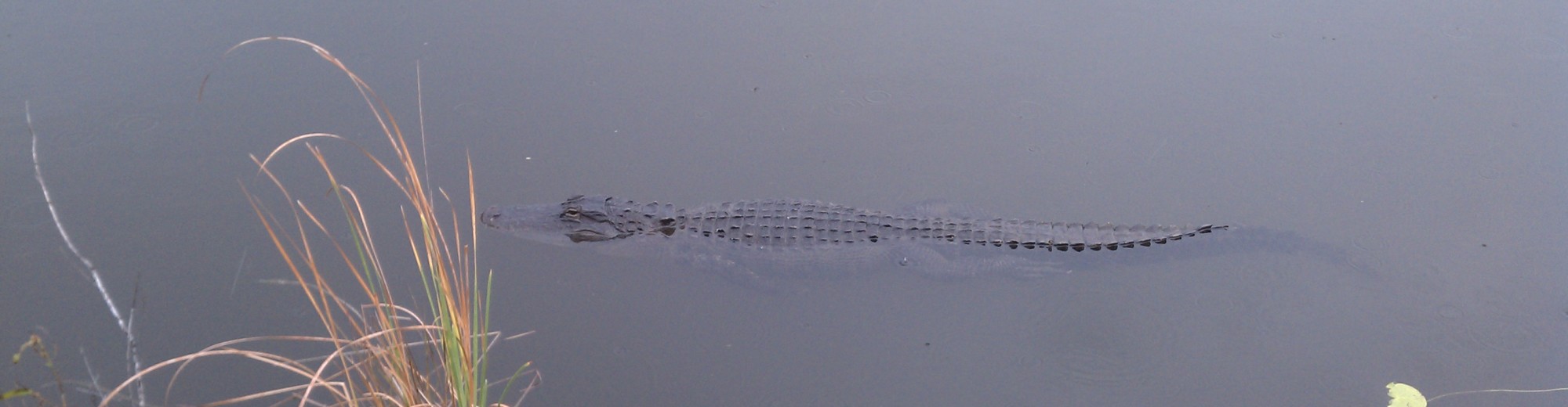
I was proctoring the final exam for my I/O Psychology course when I noticed one student (hereafter FC) behaving very strangely. FC was sitting about 3 or 4 rows from the front in the middle of the exam room, which looks like this:

2015-12-18 14.16.53

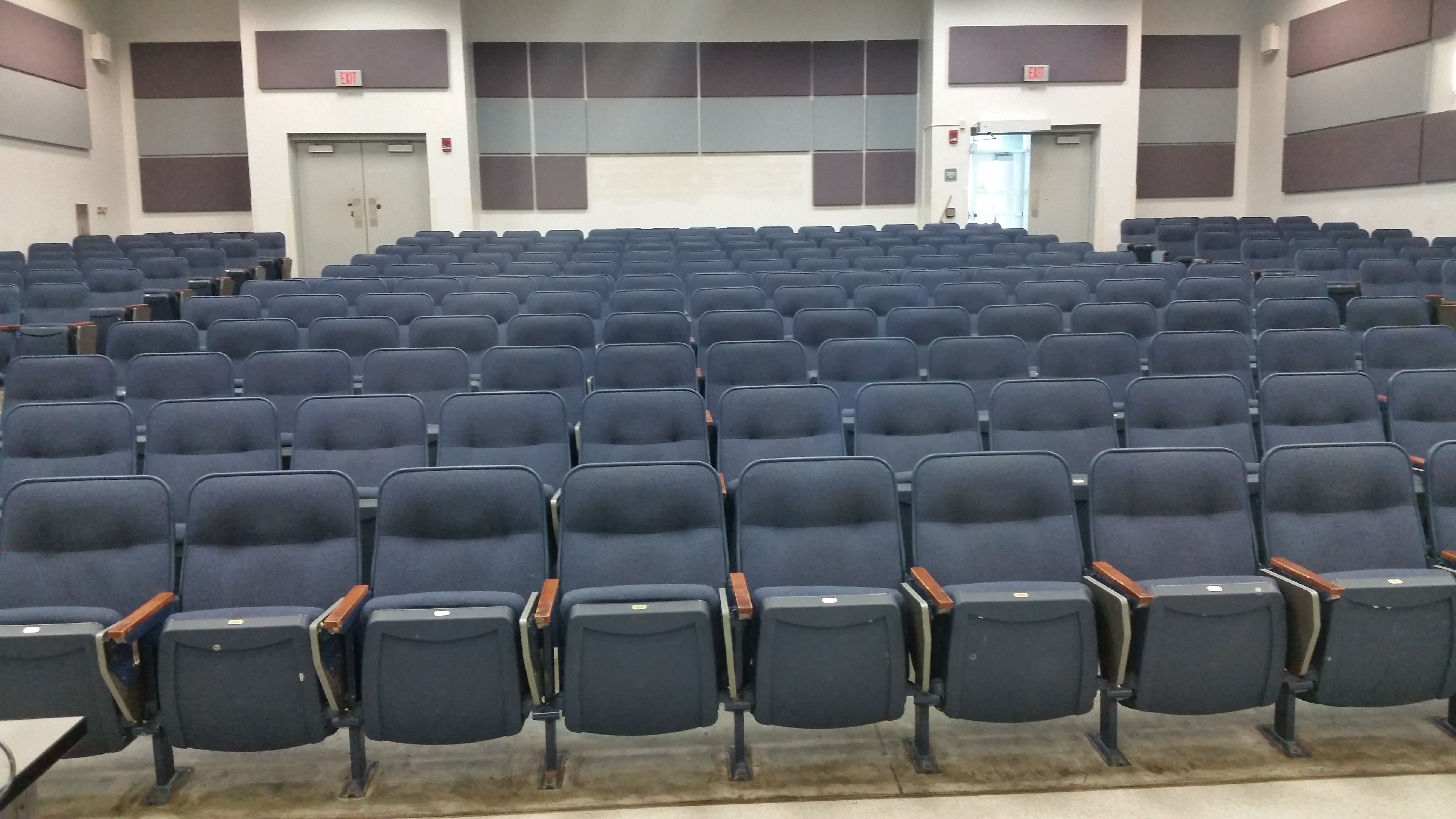
As you can see in the picture, each seat has a pullout writing table. They are designed to be on the right-hand side of the chair (facing the front of the room; sorry left-handers). That means almost everyone — when taking an exam — has their body posture turned to the right. FC was the only student in the classroom with his body posture to the left. I started watching FC more closely. In doing so, I noticed that FC was repeatedly looking to his left. And these were not just glances, but lengthy stares with head down and eyes averted. Another student (TS) was taking an exam two seats away (with the seat between them unoccupied). So I got up to take a closer look.

When I got close, I was very confused. TS had a blue exam (Form A) while FC had a green exam (Form B). I always use two forms and try to separate students so that they are not next to someone with the same form (as was the case here). Why would FC copy answers from the wrong form? (In this case, Form A and B have the same questions, but the response options are randomized.) Strange. I made a mental note to keep both exams and take a closer look once they were turned in.

TS finished first. Interestingly, after TS had finished, FC’s body posture changed to be more like everyone else. When FC turned in the exam, I was immediately 100% convinced of cheating. The giveaway was that FC — who had a green (Form B) had written “Form A” at the top of the scantron (yet placed it in the green pile). My guess is that FC assumed we would correct the “mistake” of the scantron being in the wrong pile ourselves and grade FC’s scantron using the Form A key (though I know FC physically had a copy of Form B). To add even more evidence against FC, I noticed that FC’s scantron had originally had “B” written at the top, which was erased and changed to “A.” Further, the first 10-15 answers on FC’s scantron had eraser marks. I checked the eraser marks with the Form B (FC’s original form) key and FC had marked the correct answer for just about all of them. But, now they were all erased and replaced with (mostly all) correct answers for Form A — and exactly matching TS’s scantron.

Ok. So now I knew that FC cheated on the exam. But, I started wondering, could I show this statistically? To do so, I followed the guide of the blog linked above. In what follows, I provide the R code and some of the output examining this question statistically. You can download the relevant .r file and data from here. Of course, I have replaced the students’ names, except for FC and TS.

This first block of code reads in the student response data from the .xlsx file for Form A (we’ll repeat this all again for Form B). Then it reads in the answer key and *scores* the exams. We don’t actually need the exam scores, but it is good practice to double-check these against any scores from the scantron team to be sure we are using the proper key, etc.

# Final Form A Cheating Check
library(xlsx)
library(multicon)
setwd("C:/Users/Sherman/Dropbox/Blog Posts/Cheating/")
# Read in the data
FinalExamA <- read.xlsx("Final Exam Scores.xlsx", 1)
# Get just the student responses
responsesA <- FinalExamA[,grep("Question", names(FinalExamA))]
# Bring in the answer key
answersA <- as.character(unlist(read.table("FinalFormAKey.txt",header=F)))
answersA.matrix <- matrix(answersA, nrow=nrow(responsesA), ncol=length(answersA), byrow=T)
# Score Tests and get descriptives
markedA <- responsesA==answersA.matrix
scoresA <- rowSums(markedA, na.rm=T) # na.rm to deal with missing responses
describe(scoresA)
alpha.cov(cov(markedA, use='p')) # Matches Kuder-Richardson 20

Here is the output:

> describe(scoresA)
  vars  n  mean  sd median trimmed  mad min max range  skew kurtosis   se
1    1 41 82.29 7.8     83   82.58 7.41  64  99    35 -0.22    -0.36 1.22
> alpha.cov(cov(markedA, use='p')) # Matches Kuder-Richardson 20
[1] 0.8034012

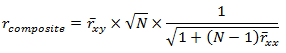
It is good to check that all of the descriptive statistics match as well as the Kuder-Richardson 20 (alpha). Now we want to compute the key scores of interest: the total number of responses matched, the total number of responses matched that were correct, and the total number of responses matched that were incorrect for EVERY pair of students with the same exam (for Form A that is 41*40 / 2 = 820 pairs). The code I used to do this is below and it looks different from Jonathan’s code because I tried to make it more efficient (by using lapply instead of for loops). I’m not sure I succeeded, but the code gets us both to the same place:

# Getting a data.frame of response matches for each pair of students
combs <- combn(FinalExamA$Student.Name, 2)
pair.list <- apply(combs, 2, function(x) responsesA[x,])
matchesA <- lapply(pair.list, function(x) x[1,]==x[2,])
sharedA <- unlist(lapply(matchesA, sum))
rightA <- unlist(lapply(pair.list, function(x) sum(x[1,]==x[2,] & x[1,]==answersA)))
wrongA <- unlist(lapply(pair.list, function(x) sum(x[1,]==x[2,] & x[1,]!=answersA)))
ids.matA <- matrix(as.vector(combs), ncol=2, byrow=T)
mydfA <- data.frame(ids.matA, sharedA, rightA, wrongA)
colnames(mydfA) <- c("SID1", "SID2", "shared", "right", "wrong")
dim(mydfaA)
head(mydfA)

And a view of the output:

> dim(mydfA)
[1] 820   5
> head(mydfA)
  SID1 SID2 shared right wrong
1   S1   S2     81    79     2
2   S1   S3     84    84     0
3   S1   S4     80    78     2
4   S1   S5     81    80     1
5   S1   S6     81    81     0
6   S1   S7     79    78     1

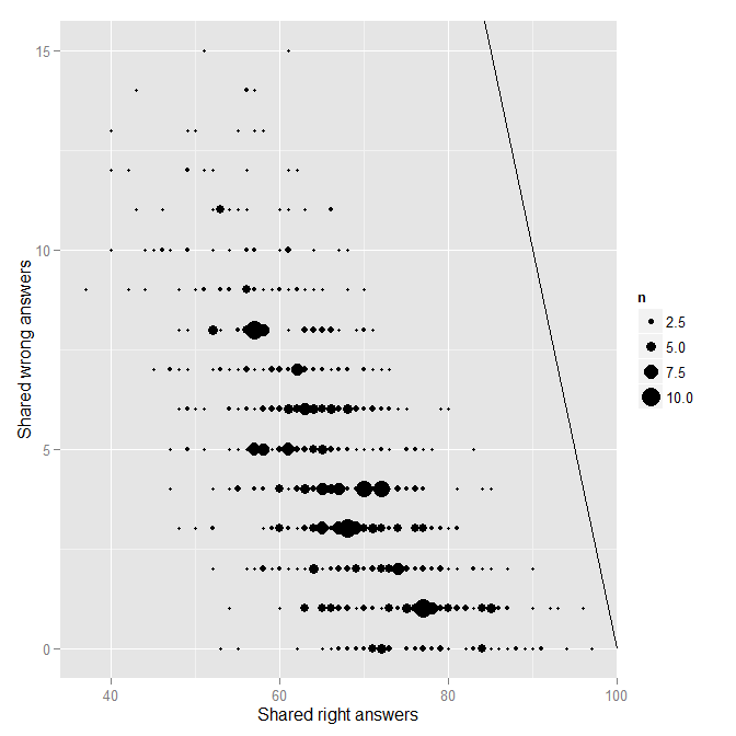
So for each pair of students, we have the number of answers they shared, the number they shared and got correct, and the number they shared and got incorrect. The next step is to plot the number of shared incorrect (wrong) as a function of the number of shared correct (right).

  # Plotting Shared Wrong answers as a function of Shared Right answers
    # Visually inspect for outliers
library(ggplot2)
g0 <- (
ggplot(mydfA, aes(x=rightA, y=wrongA))
	# + geom_point()
	+ stat_sum(aes(size=..n..))
	# + scale_size_area()
	+ geom_abline(intercept=length(answersA), slope=-1)
	+ labs(
		x = "Shared right answers"
		, y = "Shared wrong answers"
	)
	# + stat_smooth()
)
print(g0)

And the resulting image:

FormAFigure

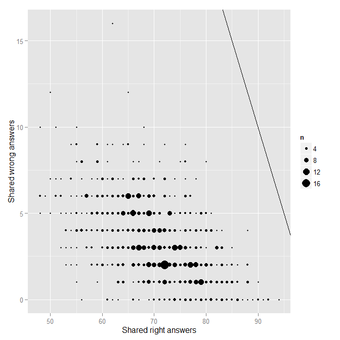
Each point on the plot represents a single pair of students. The solid black line indicates the line of “perfect matching.” No one is really near that line at all, which is good. Nonetheless, there is one obvious outlier from the rest of the distribution. Who is that pair of students near the top? You guessed it, it is FC and TS.

head(mydfA[order(mydfA$wrong, decreasing=T),])
    SID1 SID2 shared right wrong Name1 Name2
568   19   20     78    62    16    TS    FC
204    6   20     62    50    12    S6    FC
698   25   39     77    65    12   S25   S39
188    5   39     78    68    10    S5   S39
207    6   23     61    51    10    S6   S23
214    6   30     58    48    10    S6   S30

This is pretty much where Jonathan’s work on this topic stops. In thinking more about this topic though, it occurred to me that we would like some metric to quantify the degree to which the response patterns between a pair of students is an outlier (besides the visual inspection above). The simplest metric is of course the total number shared. Exams that are identical are more likely to reflect cheating. However, shared correct answers are less indicative of cheating than share incorrect answers (assuming students are actually trying to answer correctly). An alternative metric of interest is the number of shared incorrect answers given the total number of answers shared. (You can think of this as similar to a proportion. What proportion of shared answers were incorrect?) In a regression framework, we simply predict the total number of shared incorrect answers from the total number of shared answers. The pairs with large residuals indicate outliers (i.e., potential cheating pairs).

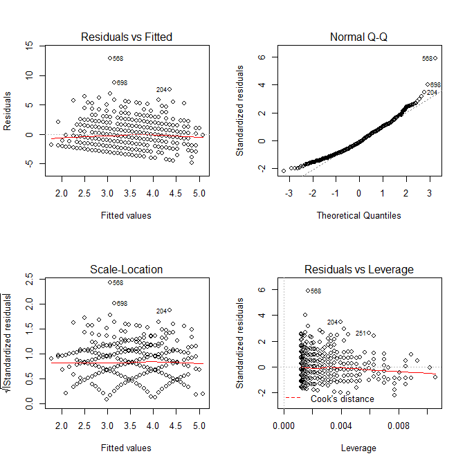
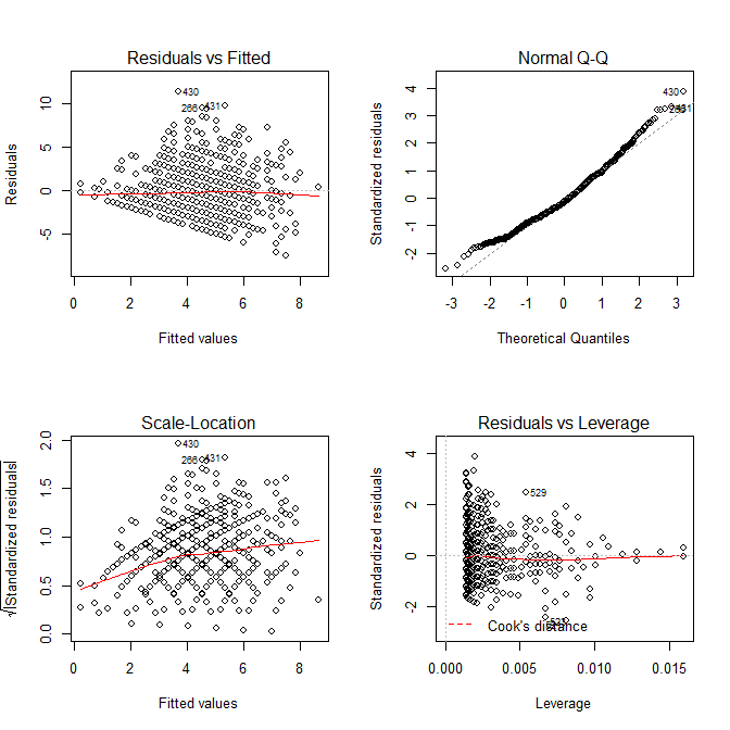
modA <- lm(wrongA ~ sharedA, data=mydfA)
sort(resid(modA)) # Sorting the residuals
op <- par(mfrow=c(2,2))
plot(modA) # Looking for outliers
hist(resid(modA), col='cyan') # Plotting the residuals

We can take advantage of the diagnostic plots provided by the plot() function to look for outliers. Note that case 568 (our case in question) is quite far from the rest of the data with a residual value of 12.94.

FormAResidualPlots

A histogram of the residuals looks like this:

FormAResidualHistogram

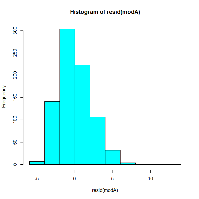
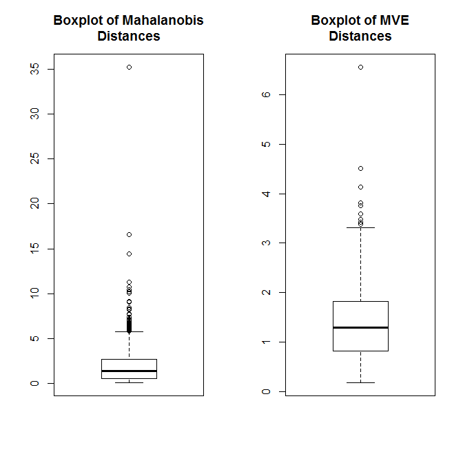
Our case in question is pretty extreme compared to the rest of the distribution. We can also use multivariate outlier detection methods to quantify the distance of each pair of X, Y points (Shared, Shared Incorrect) from the distribution’s center. The first method below here uses Mahalanobis distance and the second uses a robust outlier detection method based on the minimum volume ellipsoid (MVE). In both cases, our pair is question is clearly quite extreme.

  # A non-robust multivariate outlier detection method
mDA <- mahalanobis(mydfA[,3:4], colMeans(mydfA[,3:4]), cov(mydfA[,3:4]))
which.max(mDA)
sort(mDA)

  # A robust outlier detection method
source("http://dornsife.usc.edu/assets/sites/239/docs/Rallfun-v29.txt")
mveA <- outmve(as.matrix(mydfA[,3:4]))
which.max(mveA$dis)
sort(mveA$dis)
op <- par(mfrow=c(1,2))
boxplot(mDA, main="Boxplot of Mahalanobis\nDistances")
boxplot(mveA$dis, main="Boxplot of MVE\nDistances")

FormADistanceBoxplots

In the .r file linked, these analyses can be replicated for Form B. There is also code for combining the results for both forms into a single chart. Here I will chose show the key graphics for Form B.

FormBFigure

Note in the above that no pair of points seems all too extreme. Using the regression approach, the lack of extremity is confirmed with the diagnostic plots:

FormBResidualPlots

Ultimately, Form B looks pretty good. Nonetheless, in an effort to be very thorough, I repeated the above analyses for each of the three midterms I gave this past semester. There didn’t appear to be any issues for Midterms 1 and 2. However, one outlier did appear for Midterm 3:

Midterm3FormBFigure

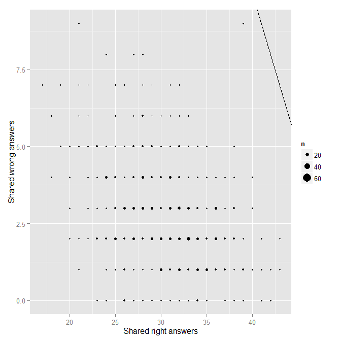
Sure enough, FC was one of the two in the pair. I happen to remember where FC was sitting for the 3rd midterm, but I do not remember where the person with whom FC’s midterm is very similar was sitting that day. I contacted the potential target student to see if he/she could recall, but I have not heard back yet.

Conclusion
What can we conclude here? On one hand, I believe that this provides at least some anecdotal validation for the method described by Jonathan Dushoff in his original post. I physically saw the student cheating and the statistical evidence confirmed my eye-witness account. However, I’m not sure if the statistical evidence alone would be grounds enough for conviction. One problem with the method is that it only identifies pairs of response patterns that look too similar. The statistics alone cannot tell you how those response patterns got similar. The obvious possibility is one student copying off of another, as we have here. However, other possibilities include (a) students working collaboratively on the exam, (b) students who study together or use the same study guide, and (c) randomness. Regarding (c), with any distribution there are bound to be extreme scores. Determining what scores are so extreme as to make randomness a remote possibility would require substantially more work. In this regard, it should be kept in mind that students who perform poorly often share incorrect answers when questions have a single strong distractor option. Regarding (b), it would be interesting to gather data from students to include indicators of studying partners / groups and using shared study guides. We can empirically investigate the question of: do people who study together have more similar exam responses than those who not? Finally, without either a confession or other physical evidence (e.g., an eye-witness, an impossibility based on the seating arrangement), the statistical evidence cannot tell you who in the pair was doing the cheating. Nonetheless, I still believe that using these sorts of tools after the fact may alert professors to the likely frequency of cheating on their exams. And at a bare minimum, the fact that professors can identify potential cheaters based on response patterns alone ought to strike fear in the hearts of those who can peek without getting caught.

What Are Situations?

Reblogged from: https://www.psychologytoday.com/blog/the-situation-lab/201507/what-are-situations

What were you doing yesterday at 10am? 2pm? 8pm? Why were you doing those things? A moment’s reflection on our day’s activities makes it obvious that situations impact our behavior. But what are situations actually? I’ve spent the past 9 years doing research aimed at answering this very question. This post reflects what we currently know about situations.

One obvious definition of a situation is that it constitutes everything that is outside the person. That is, a person is—psychologically speaking—made up of goals, motives, values, interests, skills, abilities, etc., and situations are everything else, including other people. This is, unfortunately in my view, the definition of situations that has long persisted in social psychology. When social psychologists say that “situations matter,” they are largely referring to just about anything and everything they can think of that is outside the person. They are not wrong; but this definition is a bit nebulous for anyone interested in seriously discussing the ways in which situations impact behavior, how situations can be compared across time and space, which kinds of people find themselves in one situation vs. another, and so on.

My long-time collaborators and I have worked to define three different kinds of situational information: Cues, Characteristics, and Classes.1 Cues consist of raw physical stimuli in the environment that are objective quantifiable. The number of people present, the room temperature, or the lighting are just a few examples. By definition, cues are themselves meaningless. They have also historically been useful in experimental social psychology (e.g., changing the number of people conforming; presence or absence of a social prime).

Characteristics are psychologically meaningful interpretations of situations formed from single or multiple cues once they have been implicitly or explicitly processed. Characteristics can be used to describe situations in a fashion similar to the way people can be described with personality dimensions. My colleagues and I recently proposed a taxonomy of situation characteristics that centers around 8 basic dimensions.2 The Situational Eight DIAMONDS are Duty (Does work need to be done?) Intellect (Is deep cognitive information processing required?), Adversity (Is someone under threat?), Mating (Does the situation involve romantic potential?), pOsitivity (Is the situation enjoyable?), Negativity (Could the situation cause emotional turmoil?), Deception (Can we trust each other?), and Sociality (Is meaningful social interaction and relationship building possible?). Characteristics such as the DIAMONDS allow people to communicate situational information that centers around psychological meaning.

Classes are types of situations that are grouped together because they tend to share similar constellations, or patterns, of characteristics. Religious ceremonies, parties, and work are just a few examples. Classes of situations are often useful in everyday communication because they allow people to quickly describe and exchange information about situations they have experienced. For example, if your friend tells you they were “in a meeting with the boss,” you have an idea of what that situation (work) is typically like. However, this example also demonstrates that, while situation classes can quickly convey large chunks of situational information, they often leave many important characteristics unspecified. That is, while “a meeting with the boss” almost certainly involves Duty, it is not clear if the situation also involves Intellect (does one need to think hard?), Adversity (is the boss criticizing me?), Mating (is the boss making a pass at me?), pOsitivity (am I being praised for good work?), Negativity (is information about pending layoffs looming?), Deception (can I trust what my boss is saying?), or Sociality (is it just socializing about family and life?). Thus, while classes are useful in everyday conversation, our research suggests that the most scientifically productive way to study and measure situations—if one is interested in behavioral prediction—is at the mid-level of situation characteristics.

Indeed, we have shown that situation characteristics do in fact predict behavior. In a recent study,3 we sent 56 text messages over a 1 week period to 200+ participants asking them about their current situation (at the time of the text) and their behavior in that situation. All eight of the DIAMONDS characteristics substantially predicted within-person variation (i.e., moment-to-moment change) in behavior in theoretically meaningful ways. For example, when a person was in a situation that was higher in Duty, he or she behaved in a more conscientious manner.

The foregoing discussion may leave some readers wondering: Are situations real or just inside the heads of observers? That is, if situation cues have to be interpreted to be translated into meaningful situation characteristics, aren’t situations just entirely made up? My answer to this question is unequivocally: yes and no. Yes, it is true that situation characteristics must be formed observations and interpretations of situation cues. However, it is also true that many observers readily agree about the meaning of most situations.4,5,6 This suggests that situation characteristics represent socio-cultural norms and rules. Moreover, these norms and rules have real consequences. In situations that call for work to be done, the quality and quantity of the work that is done can have a major impact on you (e.g., if you don’t do the work, you may be fired). Finally, and despite the fact that people largely agree about what situations are like, people do exhibit relatively small—but stable—individual differences in situation perception in both laboratory and real-world studies.5, 6 For example, people who are open to experience tend to see situations as more aesthetically pleasing, people who are happy tend to see more pOsitivity in situations, and people who are narcissistic tend to see themselves more as the center of attention in situations.

So to summarize, (1) situations can be described by cues, characteristics, or classes, depending on one’s research goals or level of interest, (2) situations are real—at least in their consequences—and they impact our behavior all the time, and (3) people generally agree about what a given situation is like, but individual differences in situation perception do exist and they are related to personality.


Note: I am grateful to John Rauthmann for comments on a previous draft of this post.

References

1Rauthmann, J. F., Sherman, R. A., & Funder, D. C. (2015). Principle of situation research: Towards a better understanding of psychological situations. European Journal of Personality, 29, 363-381.

2Rauthmann, J. F., Gallardo-Pujol, D., Guillaume, E. M., & Todd, E., Nave, C. S., Sherman, R. A., Ziegler, M., Jones, A. B., & Funder, D. C. (2014). The Situational Eight DIAMONDS: A taxonomy of major dimensions of situation characteristics. Journal of Personality and Social Psychology, 107, 677-718.

3Sherman, R. A., Rauthmann, J. F., Brown, N. A., Serfass, D. S., & Jones, A. B. (2015, in press). The independent effects of personality and situations on real-time expressions of behavior and emotion. Journal of Personality and Social Psychology.

4Rauthmann, J. F. (2012). You say the party is dull, I say it is lively: A componential approach to how situations are perceived to disentangle perceiver, situation, and perceiver x situation variance. Social Psychological and Personality Science, 3, 519-528.

5Serfass, D. S., & Sherman, R. A. (2013). Personality and the perceptions of situations from the Thematic Apperception Test. Journal of Research in Personality, 47, 708-718.

6Sherman, R. A., Nave, C. S., & Funder, D. C. (2013). Situational construal is related to personality and gender. Journal of Research in Personality, 46, 87-101.

Can a Computer Judge Your Personality Better than Your Friends?

Yesterday, as I was standing in line in my campus bookstore, I heard someone on the radio talk about a new study published in the Proceedings of the National Academy of Sciences (PNAS) showing that a computer algorithm, relying only on the things you “Like” on Facebook, makes more accurate judgments of your personality than your friends. If you also heard about this study, you probably did not react the way I did yesterday. Having been a reviewer on this study, I had already read the paper. So my reaction was, “Yeah, the study did show that, but it isn’t as simple as this report makes it sound.”

So what does the study show? I personally was intrigued by three things.

1) Clearly there is a sexy news story in saying that computers make better judgments than humans. And that is precisely how this study has been discussed so far.[1] However, the data show that self-other agreement with human judges was about r = .49 (across all Big 5 traits) while self-other agreement with computer-based judgments was about r = .56. Yes, these differences are statistically significant and NO we shouldn’t care that they are statistically significant. What these effectively mean is that if you judge yourself to be above average (median) on a trait, your friends are likely to guess that you are above average 74.5% of the time, while the computer algorithm guesses correctly 78% of the time. This is a real difference, so I don’t want to downplay it, but it is important not to oversell it either.

2) To me, and I noted this in my review, one of the most interesting findings from this paper was the fact that both computer-based personality judgments from Facebook Likes *AND* peer judgments of personality predicted self-reports of personality largely independently of each other. This is discussed on p. 3 of the paper in the first full paragraph under (the beautiful looking) Figure 2. You can also see the results for yourself in Supplemental Table 2 here. Average self-other agreement with human judgments was r = .42 when controlling for computer judgments. Likewise, average self-other agreement with computer judgments was r = .38 when controlling for human judgments. Both the computer algorithm and human judgments have substantial and unique contributions to self-other agreement. That is pretty cool if you ask me.

3) Although the paper and the reports make it sound as if computers have some sort of knowledge that we do not, this is of course not true. The computer-based algorithm for making personality judgments is based entirely on the person’s behavior. That is, “Liking” something on Facebook is a behavior. The computer is taking the sum total of those behaviors into account and using them as a basis for “judgment.” And these behaviors came from the person whose personality is being judged. Thus, one could argue that the computer judgments are merely linking self-reports of behavior or preferences (e.g., I like Starbucks) with self-reports of personality.

I don’t mean to downplay the study here. I thought it was a really interesting and well-conducted study when I reviewed it, and I still do. The study combines a large sample, multiple methodologies, and sophisticated (but appropriate) analytic techniques to examine something really interesting. In those respects, this study is a model for how many of us should be doing psychological research.

[1] All I did was Google “computers are better than humans” and those were the top three stories to appear. I’m told there are many more.

Note: Thanks to David Funder and Simine Vazire for prior comments on this post.

Developing Short Measures of Broad Constructs: Issues of Reliability and Validity

Consider the following problem. I have a 4-item measure of a psychological construct. Let’s call it Extraversion. Here are the four items:

  • I like to go to parties
  • I am a talkative person
  • I see myself as a good leader
  • I like to take charge

It might be obvious to some, but the first two items and the last two items are more related to each other than the other combinations of items. In fact, we could say the first two items measure the “Sociability” aspect of Extraversion while the last two items measure the “Assertiveness” aspect of Extraversion.

Now let’s say I am in a real bind because, although I love my 4-item measure of Extraversion, in my next study I only have time for a 2-item measure. Which two items should I choose?

Let’s further say that I have collected a lot of data using our 4-item measure and know that the correlation matrix among the items looks like this:

Item 1 Item 2 Item 3 Item 4
Item 1 1.00 .80 .30 .30
Item 2 1.00 .30 .30
Item 3 1.00 .80
Item 4 1.00


So as noted above, the first two items and the last two items are highly correlated, but all items are at least moderately associated. So which two items should I choose?

The Case for High Internal Consistency

At some point, almost every psychology student is taught that reliability limits validity. That is, on average, the correlation between two constructs cannot exceed the square root of the product of their reliabilities. Or more simply, scales with higher reliability can achieve higher validity. The most frequently used method of estimating reliability is undoubtedly Cronbach’s alpha. Cronbach’s alpha is a measure of the internal consistency of a scale (assuming a single factor underlies the scale). Cronbach’s alpha is also an estimate of reliability under the special condition that the items making up the scale can be thought of as a random subset of the population of items that could make up the scale. With this in mind, the obvious choices are to go with either Items 1 and 2 or Items 3 and 4. Either of those combinations will certainly have higher internal consistency in our new study.

The Case for Content Coverage

However, if we select one of the high internal consistency options, we are sacrificing content coverage in our measure. Indeed, one could easily argue that our shorter measure is now either a measure of Sociability or Assertiveness, but not Extraversion. From a logical standpoint, if we want to cover our entire construct, we should choose those items that are the least correlated with each other (in this case that any of the following combinations: 1_3, 1_4, 2_3, or 2_4). Unfortunately, all of these choices are going to have lower internal consistencies. And as noted above, a low reliability will limit our validity. Or will it?

I’ve created an example in R to work through this hypothetical, but relatively realistic, problem. Let’s first begin by creating our population correlation matrix. We will then use that population correlation matrix to generate some random data to test out our different options. Of course, because we want to examine validity, we need some sort of criterion. So to our matrix from above, I’ve added a fifth variable – let’s call it popularity – and I’m assuming this variable correlates r = .10 with each of our items (i.e., has some small degree of validity).


library(mvtnorm)

mat <- matrix(c(1,.8,.3,.3,.1,

.8,1,.3,.3,.1,

.3,.3,1,.8,.1,

.3,.3,.8,1,.1,

.1,.1,.1,.1,1),

ncol=5, byrow=T)

set.seed(12345) # See we can get the same results

dat <- rmvnorm(n=10000, sigma=mat)

cor(dat[,1:4]) # Our sample correlation matrix for our key items

[,1] [,2] [,3] [,4]

[1,] 1.0 0.8 0.3 0.3

[2,] 0.8 1.0 0.3 0.3

[3,] 0.3 0.3 1.0 0.8

[4,] 0.3 0.3 0.8 1.0

As noted above, there are six possible combinations of items to form composites we could choose from: 1_2, 1_3, 1_4, 2_3, 2_4, and 3_4. One thing that might tip our decision about which to use is to first determine which combination of items correlates most closely with the scores we would get from our 4-item measure. The partwhole() function in the {multicon} package does this for us rapidly:


library(multicon)

partwhole(dat[,1:4], nitems=2)

The argument nitems=2 tells the function that we want to look at all of the possible 2-item combinations. The results look like this (note I’ve rounded them here):


1_2 1_3 1_4 2_3 2_4 3_4

Umatch 0.82 0.96 0.96 0.96 0.96 0.82

Fmatch 0.81 0.96 0.96 0.96 0.96 0.82

The top row (1_2, 1_3, etc.) identifies the combination of items that was used to form a composite. The next row (Umatch) are the partwhole correlations between the scores for that two-item composite, using unit weighting, and the total scores yielded by averaging all four items. The third row (Fmatch) contains the partwhole correlations between the scores for that two-item composite, using component scores, and the total scores yielded from a single principle component of all four items. The numbers are very similar across rows, but in this case we care more about Umatch because we intend on creating a unit-weighted composite with our new measure.

What should be obvious from this pattern of results is that the four combinations of items that select one item from each aspect (Sociability and Assertiveness) have much stronger partwhole correlations than either of the other two (more internally consistent) combinations.

What about internal consistency? We can get the internal consistency (alpha) for our four-item measure and for each possible combination of two items measures:


alpha.cov(cor(dat[,1:4]))

# For various combinations of 2 items

alpha.cov(cor(dat[,1:2]))

alpha.cov(cor(dat[,c(1,3)]))

alpha.cov(cor(dat[,c(1,4)]))

alpha.cov(cor(dat[,2:3]))

alpha.cov(cor(dat[,c(2,4)]))

alpha.cov(cor(dat[,3:4]))

The internal consistencies are .78 for the 4-item measure, .89 for the two Sociability items and .88 for the two Assertiveness items. Those are fairly high and fall into what many psychologists might call the “acceptable” range for reliability. The other four combinations do not fare so well with reliabilities of .46. Many people would consider these “unacceptably low.” So clearly, combinations 1_2 and 3_4 are the winners from an internal consistency standpoint.

But what about validity? Arguably, the entire point of the scientific enterprise is validity. Indeed, some might argue that the whole point of measurement is prediction. So how do our six combinations of 2-item scales do in terms of predicting our criterion?

We can use the scoreTest() function, available in the {multicon} package[1], to create our six composite scores.


myKeys <- list(OneTwo = c(1,2), OneThree = c(1,3), OneFour = c(1,4),

TwoThree = c(2,3), TwoFour = c(2,4), ThreeFour = c(3,4))

out <- scoreTest(data.frame(dat), myKeys, rel=TRUE)

out$rel # The same alphas as before with more information

describe(out$scores)

Note that scoreTest() has an option for calculating the alphas (and other metrics of internal consistency). You can check those for consistency with the above.

Now let’s correlate our six composites with the criterion. But beyond these validity coefficients, we might also want to look at the validities if we correct for attenuation. We can do the latter by simply dividing the observed correlations by the square root of their estimated reliabilities (internal consistencies).


ObsCors <- cor(out$scores, dat[,5])

DisCors <- ObsCors / sqrt(out$rel[,1])

# Which combination is best as predicting the criterion?

round(data.frame("r"=ObsCors, "rho"=DisCors),2)

r rho

OneTwo   0.10 0.11

OneThree 0.12 0.18

OneFour   0.13 0.19

TwoThree 0.12 0.17

TwoFour   0.12 0.18

ThreeFour 0.11 0.11

So how do our results look? First in terms of observed correlations (r), the constructs that used one item from Sociability and Assertiveness outperform the constructs that use only Sociability or Assertiveness items. The picture is even clearer when we look at the corrected correlations (rho). By virtue of their high internal consistencies, neither the pure Sociability nor the pure Assertiveness composites gain much when corrected for unreliability.

So it seems, in regards to our hypothetical case here, we should prefer any combination of items that uses one Sociability and one Assertiveness item when creating our new 2-item measure of Extraversion. This might seem counterintuitive to some. To others, this might seem obvious. And actually, Guilford (1954) showed this a long time ago in his equation 14.37:

GuilfordEq

In this equation, rcomposite is the validity of a composite of N items, rxy is the average validity of each item in the composite, and rxx is the average inter-correlation of the items forming the composite. The simple R script below applies Guilford’s equation to our situation.


# Applying Guilford's Equation

AvgItemValidities <- rep(.1, 6)

NItems <- 2

AvgItemCors <- c(.8,.3,.3,.3,.3,.8)

&nbsp;

guilford <- function(rXY, N, rXX) {

return(rXY * sqrt(N) * 1 / sqrt(1 + (N - 1)*rXX))

}

round(guilford(AvgItemValidities, NItems, AvgItemCors),3)

[1] 0.105 0.124 0.124 0.124 0.124 0.105

And the results are almost dead-on with what our simulation shows. That is, holding the number of items and the average validity of the items constant, increased internal consistency decreases composite validity. I’m not sure how many people know this. And amongst those who do, it is not clear to me how many people appreciate this fact.

Finally, to those who think this seems obvious, let me throw one more wrinkle at you. In measurement contexts (i.e., scale development) confirmatory factor analysis (CFA) is a common practice. Many people, especially reviewers, hold CFA fit results in high esteem. That is, if the model shows poor fit, it is invalid. Now, with a two-item measure, we cannot conduct a CFA because we do not have enough degrees of freedom. However, if we conduct “mental CFAs” for each of our six possible composite measures, it is obvious that model 1_2 and model 3_4 will show much better fits (i.e., they will have smaller residuals) than any of the other models. We could actually demonstrate this if we extended our example to six items and attempted to make a shorter 3-item measure. Thus, I suspect that even though much of what I said above might seem obvious to some, I also suspect that many would miss the fact that a poor CFA fit does not necessarily mean that the construct(s) being measured have poor validity. In fact, it is very possible that constructs formed from better fitting CFAs have worse predictive validity than constructs from worse fitting CFAs.

[1] This function is only available in version >=1.5 of the{multicon} package released after 1/8/2015. If you have an older version, you may need to update.

Reference

Guilford, J. P. (1954). Psychometric Methods (2nd ed.). New York: McGraw-Hill.

Note: I am grateful to Tal Yarkoni for his feedback on a prior draft of this post.

(Mis)Interpreting Confidence Intervals

In a recent paper Hoekstra, Morey, Rouder, & Wagenmakers argued that confidence intervals are just as prone to misinterpretation as tradiational p-values (for a nice summary, see this blog post). They draw this conclusion based on responses to six questions from 442 bachelor students, 34 master students, and 120 researchers (PhD students and faculty). The six questions were of True / False format and are shown here (this is taken directly from their Appendix, please don’t sue me; if I am breaking the law I will remove this without hesitation):

Bubledorf

Hoekstra et al. note that all six statements are false and therefore the correct response to mark each as False. [1] The results were quite disturbing. The average number of statements marked True, across all three groups, was 3.51 (58.5%). Particularly disturbing is the fact that statement #3 was endorsed by 73%, 68%, and 86% of bachelor students, master students, and researchers respectively. Such a finding demonstrates that people often use confidence intervals simply to revert back to NHST (i.e., if the CI does not contain zero, reject the null).

However, it was questions #4 and #5 that caught my attention when reading this study. The reason they caught my attention is because my understanding of confidence intervals told me they are correct. However, the correct interpretation of a confidence interval, according to Hoekstra et al., is “If we were to repeat the experiment over and over, then 95% of the time the confidence intervals contain the true mean.” Now, if you are like me, you might be wondering, how is that different from a 95% probability that the true mean lies between the interval? Despite the risk of looking ignorant, I asked that very question on Twitter:

TwitterPic

Alexander Etz (@AlexanderEtz) provided an excellent answer to my question. His post is rather short, but I’ll summarize it here anyway: from a Frequentist framework (under which CIs fall), one cannot assign a probability to a single event, or in this case, a single CI. That is, the CI either contains μ (p = 1) or it does not (p = 0), from a Frequentist perspective.

Despite Alexander’s clear (and correct) explanation, I still reject it. I reject it on the grounds that it is practically useful to think of a single CI as having a 95% chance of containing μ. I’m not alone here. Geoff Cumming also thinks so. In his book (why haven’t you bought this book yet?) on p. 78 he provides two interpretations for confidence intervals that match my perspective. The first interpretation is “One from the Dance of CIs.” This interpretation fits precisely with Hoekstra et al.’s definition. If we repeated the experiment indefinitely we would approach an infinite number of CIs and 95% of those would contain μ. The second interpretation (“Interpret our Interval”) says the following:

It’s tempting to say that the probability is .95 that μ lies in our 95% CI. Some scholars permit such statements, while others regard them as wrong, misleading, and wicked. The trouble is that mention of probability suggests μ is a variable, rather than having a fixed value that we don’t know. Our interval either does or does not include μ, and so in a sense the probability is either 1 or 0. I believe it’s best to avoid the term “probability,” to discourage any misconception that μ is a variable. However, in my view it’s acceptable to say, “We are 95% confidence that our interval includes μ,” provided that we keep in the back of our minds that we’re referring to 95% of the intervals in the dance including μ, and 5% (the red ones) missing μ.

So in Cumming’s view, question #4 would still be False (because it misleads one to thinking that μ is a variable), but #5 would be True. Regardless, it seems clear that there is some debate about whether #4 and #5 are True or False. My personal belief is that it is okay to mark them both True. I’ve built a simple R example to demonstrate why.

# First, create 1000 datasets of N=100 each from a normal distribution.
set.seed(5)
sims <- 1000
datasets <- list()
for(i in 1:sims) {
  datasets[[i]] <- rnorm(100)
}

  # Now get the 95% confidence interval for each dataset.
out <- matrix(unlist(lapply(datasets, function(x) t.test(x)$conf.int)), ncol=2, byrow=T)
colnames(out) <- c("LL", "UL")
  # Count the number of confidence intervals containing Mu
res <- ifelse(out[,1] <= 0 & out[,2] >= 0, 1, 0)
sum(res) / sims
  # Thus, ~95% of our CIs contain Mu

This code creates 1000 datasets of N=100 by randomly drawing scores from a normal distribution with μ = 0 and σ = 1. It then computes a 95% confidence interval for the mean for each dataset. Lastly, it counts how many of those contain μ (0). In this case, it is just about 95%.[2] This is precisely the definition of a confidence interval provided by Hoekstra et al. If we repeat an experiment many times, 95% of our confidence intervals should contain μ. However, if we were just given one of those confidence intervals (say, at random) there would also be a 95% chance it contains μ. So if we think of our study, and its confidence interval, as one of many possible studies and intervals, we can be 95% confident that this particular interval contains the population value.

Moreover, this notion can be extended beyond a single experiment. That is, rather than thinking about repeating the same experiment many times, we can think of all of the different experiments (on different topics with different μs) we conduct and note that 95% of them will contain μ within the confidence interval, but 5% will not. Therefore, while I (think) I understand and appreciate why Hoekstra et al. consider the answers to #4 and #5 to be False, I disagree. I think that they are practically useful interpretations of a CI. If it violates all that is statistically holy and sacred, then damn me to statistical hell.

Despite this conclusion, I do not mean to undermine the research by Hoekstra et al. Indeed, my point has little bearing on the overall conclusion of their paper. Even if questions #4 and #5 were removed, the results are still incredibly disturbing and suggest that we need serious revisions to our statistical training.


[1] The last sentence of the instructions makes it clear that it is possible that all True and all False are possibilities. How many people actually believed that instruction is another question.

[2] Just for fun, I also calculated the proportion of times a given confidence interval contains the sample mean from a replication. The code you can run is below, but the answer is about 84.4%, which is close to Cummings’ (p. 128) CI Interpretation 6 “Prediction Interval for a Replication Mean” of 83%.

  # Now get the sample Means
Ms <- unlist(lapply(datasets, mean))
    # For each confidence interval, determine how many other sample means it captured
reptest <- sapply(Ms, function(x) ifelse(out[,1] <= x & out[,2] >= x, 1, 0))
      # Remove the diagonal to avoid double-counting
diag(reptest) <- NA
      # Now summarize it:
mean(colMeans(reptest, na.rm=T)) # So ~ 84.4% chance of a replication falling within the 95% CI


When Are Direct Replications Necessary?

We are told that replication is the heart of all sciences. As such, psychology has recently seen numerous calls for direct replication. Sanjay Srivastava says that replication provides an opportunity to falsify an idea (an important concept in science, but rarely done in psychology). Brian Nosek and Jeffrey Spies suggest that replication would help identify “manufactured effects” rapidly. And Brent Roberts proposed a three step process, the last of which is a direct replication of any unique study reported in the package of studies.

Not everyone thinks that direct replications are useful though. Andrew Wilson has argued that replication will not save psychology and better theories are needed. Jason Mitchell has gone so far as to say that failed replications offer nothing to science as they are largely the result of practical mistakes on the part of the experimenters. So are direct replications necessary? My answer is a definitive: sometimes.

Let’s start by considering what I gather to be some of the main arguments for direct replications.

  • You might have screwed up the first study. This is one of the reasons Brent Roberts has proposed direct replications (see his response to my comment). Interestingly, this is the other side of the argument posed by Mitchell. That is, you could have typos in your measures, left questions off the survey, the coffee maker could have interfered with the EEG readings,[1] or the data could have been mishandled.
  • Direct replications, when combined with meta-analysis, yield more precise effect size estimates. What is better than one study with N=50? How about two studies with N=50 in each! Perspectives on Psychological Science is now accepting registered replication reports and one of the motivating principles is that “Direct replications are necessary to estimate the true size of an effect.” Likewise, Sean Mackinnon says “It is only through repeated experiments that we are able to center on an accurate estimate of the effect size.”
  • Direct replications can improve generalizability. All other things being equal, we would like our results to generalize to the largest group of people possible. If a study yields the expected results only when conducted on University of Michigan undergrads, we would not be so impressed. Direct replications by different investigators, in different locations, sampling from different sub-populations can offer critical information about generalizability.

But there are problems with these arguments:

  • You might have screwed up the first study. Yes, there may have been methodological problems and artifacts in the first study. But how is running a direct replication supposed to fix this problem?

My guess is that most modern labs gather data in a similar fashion to the way we gather data in my lab. One of my (super smart) graduate students logs into our survey software (we use Qualtrics) and types the survey in there, choosing the scale points, entering anchors, etc. We go through the survey ourselves checking for errors. Then we have Research Assistants do the same. Then we gather say N=5 data points (these data points are usually from members of the research team) and download the data to make sure we understand how the software is storing and returning the values we gave it. Then we run the study. Now, when it comes time to do another study do we start all over again? No. We simply click “copy survey” and the software makes a copy of the same survey we already used for another study. We can do that with lots of different surveys to the point that we almost never have to enter a survey by hand again.

Now these are not direct replications we are running. These are new studies using the same measures. But if we were running a direct replication, how would the process be different? It would be even worse because we wouldn’t even create anything new. We would just have new participants complete the same Qualtrics survey we created before noting which participants were new. So if we screwed up the measures the first time, they are still screwed up now.

Is this a new-age internet survey problem? I doubt it. When I was an undergraduate running experiments we essentially did the same thing only with paper copies. So if the anchor was off the first time someone created the survey (and no one noticed it), it was going to be off on every copy of that survey. And if we were running a direct replication, we wouldn’t start from scratch. We would just print out another copy of the same flawed survey.

Here is the good news though. With Open Science everyone can see what measures I used and how I screwed them up. Further, with open data everyone can see how the data were (mis)handled and if coffee makers created implausible outliers. Moreover, with scripted statistical analysis languages like R everyone can reproduce my results and see exactly where I screwed up the analysis (you can’t do that with point-and-click SPSS!).

Direct replications are not the solution to the problem of methodological/statistical flaws in the first study; Open Science is.

  • Direct replications, when combined with meta-analysis, yield more precise effect size estimates. This is absolutely 100% correct. It is also absolutely 100% unnecessary.

Consider three scenarios: (a) one study with n=20, (b) one study with n=400, (c) 20 studies with n=20 in each that are meta-analytically combined. Which of these will yield the most precise effect size estimate? Obviously it isn’t (a), but what about between (b) and (c)? This was precisely the topic of a post by Felix Schönbrodt. In it, Felix showed empirically that the precision of (b) and (c) are identical. While his post has great insights about precision, the empirical demonstration was (sorry Felix!) a bit useless. The mathematics of meta-analysis are some of the simplest in psychology and it is trivial to show that the standard error of an effect size based on N=400 is the same as one based on…errr, N=400.

So to put this bluntly, if we are interested in more precise effect sizes (and I think we should be), we don’t need direct replications. We need larger initial studies. Indeed, Schönbrodt and Perugini (2013) suggested that stable effect size estimates result when N=250.[2] If editors and reviewers considered sample size a more important criterion for publication there would be (a) fewer Type I errors in the literature, and (b) more precise effect size estimates (i.e., less over-estimated effect sizes due to publication bias). To underscore this point, consider the recent Facebook experiment that received much attention. The study had a total sample of N=689,003. On the scale of r the effect size estimates have a margin of error of ± .002. In one blog post about the study someone commented that the worst part is that because Facebook is so dominant in the SNS market that no one else will be able to replicate it to see if the effect really exists.[3] Seriously?!? Sorry. This study does not need to be directly replicated. The effect size estimates are pretty precise.

  • Direct replications can improve generalizability. YES! Direct replications are incredibly useful for improving generalizability.

The final argument for direct replications is to improve generalizability. This is the only reason that anyone should[4] call for direct replications. If I run a study on undergraduate students in south Florida (even with a large sample), you should in fact wonder if these results generalize to working adults in south Florida and to people from places all over the world. We probably have intuitions about which studies are likely to generalize and which ones aren’t, so we might rely on those to determine which studies are in most need of replication (for generalization purposes!). Or we might focus on trying to replicate studies that, if they are generalizable, would have the most practical and theoretical impact. I’d also suggest that we should periodically try to replicate important studies conducted some time ago (e.g., 20 years or more) just to be sure that the results generalize to modern people.

So to summarize, if we conduct good research in the first place, then we should[5] only need direct replications for generalizability purposes. If we find an error in a previously conducted study, then we should fix it. If that means running a new study with the error fixed, fine. But that isn’t a replication. It is a different (unflawed) study. And if we have good studies to begin with, we don’t need meta-analyses to provide more precise effect size estimates; we will already have them.

So, what constitutes a good study? We all probably have our own ideas, but I will provide my own personal criteria for study quality in another blog post.


[1] I have no idea if coffee makers can interfere with EEG machines. I don’t drink coffee.

[2] I think N=200 is a better number, but that is the subject of another blog post to come in the future (and also Simine Vazire’s suggestion!).

[3] I wish I had recorded the post and comment, but I didn’t. You’ll just have to take my word that it existed and I read it.

[4] I really want to emphasize should here because this is my fantasy-land where researchers actually care about precisely measuring natural relationships. If actions speak louder than words, we know that much research in psychology has little interest in precisely measuring natural relationships.

[5] See footnote 4. Please also note that I am only referring to direct replications here, not conceptual replications or extensions. Indeed, conceptual replications and extensions are crucial ways of demonstrating generalizability.

phack: An R Function for Examining the Effects of p-hacking

Imagine you have a two group between-S study with N=30 in each group. You compute a two-sample t-test and the result is p = .09, not statistically significant with an effect size r = .17. Unbeknownst to you there is really no relationship between the IV and the DV. But, because you believe there is a relationship (you decided to run the study after all!), you think maybe adding five more subjects to each condition will help clarify things. So now you have N=35 in each group and you compute your t-test again. Now p = .04 with r = .21.

If you are reading this blog you might recognize what happened here as an instance of p-hacking. This particular form (testing periodically as you increase N) of p-hacking was one of the many data analytic flexibility issues exposed by Simmons, Nelson, and Simonshon (2011). But what are the real consequences of p-hacking? How often will p-hacking turn a null result into a positive result? What is the impact of p-hacking on effect size?

These were the kinds of questions that I had. So I wrote a little R function that simulates this type of p-hacking. The function – called phack – is designed to be flexible, although right now it only works for two-group between-S designs. The user is allowed to input and manipulate the following factors (argument name in parentheses):

  • Initial Sample Size (initialN): The initial sample size (for each group) one had in mind when beginning the study (default = 30).
  • Hack Rate (hackrate): The number of subjects to add to each group if the p-value is not statistically significant before testing again (default = 5).
  • Population Means (grp1M, grp2M): The population means (Mu) for each group (default 0 for both).
  • Population SDs (grp1SD, grp2SD): The population standard deviations (Sigmas) for each group (default = 1 for both).
  • Maximum Sample Size (maxN): You weren’t really going to run the study forever right? This is the sample size (for each group) at which you will give up the endeavor and go run another study (default = 200).
  • Type I Error Rate (alpha): The value (or lower) at which you will declare a result statistically significant (default = .05).
  • Hypothesis Direction (alternative): Did your study have a directional hypothesis? Two-group studies often do (i.e., this group will have a higher mean than that group). You can choose from “greater” (Group 1 mean is higher), “less” (Group 2 mean is higher), or “two.sided” (any difference at all will work for me, thank you very much!). The default is “greater.”
  • Display p-curve graph (graph)?: The function will output a figure displaying the p-curve for the results based on the initial study and the results for just those studies that (eventually) reached statistical significance (default = TRUE). More on this below.
  • How many simulations do you want (sims). The number of times you want to simulate your p-hacking experiment.

To make this concrete, consider the following R code:

res <- phack(initialN=30, hackrate=5, grp1M=0, grp2M=0, grp1SD=1, grp2SD=1, maxN=200, alpha=.05, alternative="greater", graph=TRUE, sims=1000)

This says you have planned a two-group study with N=30 (initialN=30) in each group. You are going to compute your t-test on that initial sample. If that is not statistically significant you are going to add 5 more (hackrate=5) to each group and repeat that process until it is statistically significant or you reach 200 subjects in each group (maxN=200). You have set the population Ms to both be 0 (grp1M=0; grp2M=0) with SDs of 1 (grp1SD=1; grp2SD=1). You have set your nominal alpha level to .05 (alpha=.05), specified a direction hypothesis where group 1 should be higher than group 2 (alternative=“greater”), and asked for graphical output (graph=TRUE). Finally, you have requested to run this simulation 1000 times (sims=1000).

So what happens if we run this experiment?* So we can get the same thing, I have set the random seed in the code below.

source("http://rynesherman.com/phack.r") # read in the p-hack function
set.seed(3)
res <- phack(initialN=30, hackrate=5, grp1M=0, grp2M=0, grp1SD=1, grp2SD=1, maxN=200, alpha=.05, alternative="greater", graph=TRUE, sims=1000)

The following output appears in R:

Proportion of Original Samples Statistically Significant = 0.054
Proportion of Samples Statistically Significant After Hacking = 0.196
Probability of Stopping Before Reaching Significance = 0.805
Average Number of Hacks Before Significant/Stopping = 28.871
Average N Added Before Significant/Stopping = 144.355
Average Total N 174.355
Estimated r without hacking 0
Estimated r with hacking 0.03
Estimated r with hacking 0.19 (non-significant results not included)

The first line tells us how many (out of the 1000 simulations) of the originally planned (N=30 in each group) studies had a p-value that was .05 or less. Because there was no true effect (grp1M = grp2M) this at just about the nominal rate of .05. But what if we had used our p-hacking scheme (testing every 5 subjects per condition until significant or N=200)? That result is in the next line. It shows that just about 20% of the time we would have gotten a statistically significant result. So this type of hacking has inflated our Type I error rate from 5% to 20%. How often would we have given up (i.e., N=200) before reaching statistical significance? That is about 80% of the time. We also averaged 28.87 “hacks” before reaching significance/stopping, averaged having to add N=144 (per condition) before significance/stopping, and had an average total N of 174 (per condition) before significance/stopping.

What about effect sizes? Naturally the estimated effect size (r) was .00 if we just used our original N=30 in each group design. If we include the results of all 1000 completed simulations that effect size averages out to be r = .03. Most importantly, if we exclude those studies that never reached statistical significance, our average effect size r = .19.

This is pretty telling. But there is more. We also get this nice picture:

phackPic

It shows the distribution of the p-values below .05 for the initial study (upper panel) and for those p-values below .05 for those reaching statistical significance. The p-curves (see Simonsohn, Nelson, & Simmons, 2013) are also drawn on. If there is really no effect, we should see a flat p-curve (as we do in the upper panel). And if there is no effect and p-hacking has occurred, we should see a p-curve that slopes up towards the critical value (as we do in the lower panel).

Finally, the function provides us with more detailed output that is summarized above. We can get a glimpse of this by running the following code:

head(res)

This generates the following output:

   Initial.p  Hackcount     Final.p  NAdded    Initial.r       Final.r
1 0.86410908         34  0.45176972     170  -0.14422580   0.006078565
2 0.28870264         34  0.56397332     170   0.07339944  -0.008077691
3 0.69915219         27  0.04164525     135  -0.06878039   0.095492249
4 0.84974744         34  0.30702946     170  -0.13594941   0.025289555
5 0.28048754         34  0.87849707     170   0.07656582  -0.058508736
6 0.07712726         34  0.58909693     170   0.18669338  -0.011296131

The object res contains the key results from each simulation including the p-value for the initial study (Initial.p), the number of times we had to hack (Hackcount), the p-value for the last study run (Final.p), the total N added to each condition (NAdded), the effect size r for the initial study (Initial.r), and the effect size r for the last study run (Final.r).

So what can we do with this? I see lots of possibilities and quite frankly I don’t have the time or energy to do them. Here are some quick ideas:

  • What would happen if there were a true effect?
  • What would happen if there were a true (but small) effect?
  • What would happen if we checked for significance after each subject (hackrate=1)?
  • What would happen if the maxN were lower?
  • What would happen if the initial sample size was larger/smaller?
  • What happens if we set the alpha = .10?
  • What happens if we try various combinations of these things?

I’ll admit I have tried out a few of these ideas myself, but I haven’t really done anything systematic. I just thought other people might find this function interesting and fun to play with.

* By the way, all of these arguments are set to their default, so you can do the same thing by simply running res <- phack()


Update (10/11/2014) phackRM() is now available at http://rynesherman.com/phackRM.r to simulate p-hacking for dependent samples.