Some months ago I came across this blog post by Jonathan Dushoff discussing some statistical procedures for detecting cheating (e.g., copying, working together) on multiple choice exams. The method is quite elegant and the post is fairly short so you may wish to read that post. After reading about this method, I considered applying it to my old exams. In my undergraduate courses I typically give 3 midterms (50 questions each; with either 3 or 4 response options) and 1 final exam (100 questions). The exams are done using scantrons, meaning that students indicate their answers on a standardized form which is then read by a computer to detect their responses. Their responses are then compared to an answer key, scoring their exams. The scantron folks here at FAU provide the professors with a .xlsx file containing the responses the computer recorded for each student on each question. With such a file in hand, it is fairly easy to apply the code provided by Jonathan with a bit of extra work (e.g., inputting the exam key). Despite the relative ease with which this could be done, I really wasn’t that motivated to do this sort of work. That all changed a few weeks ago.
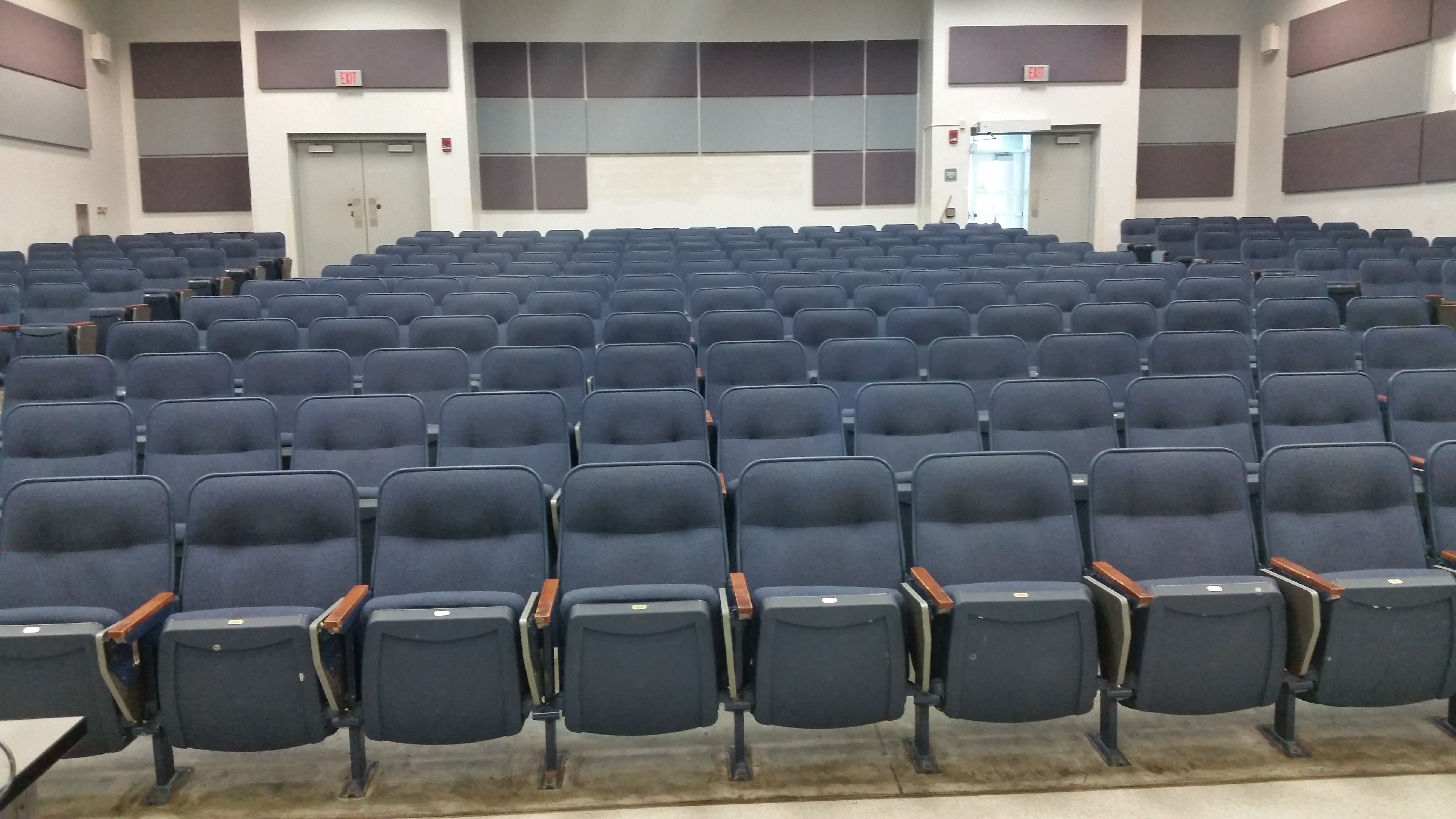
I was proctoring the final exam for my I/O Psychology course when I noticed one student (hereafter FC) behaving very strangely. FC was sitting about 3 or 4 rows from the front in the middle of the exam room, which looks like this:
As you can see in the picture, each seat has a pullout writing table. They are designed to be on the right-hand side of the chair (facing the front of the room; sorry left-handers). That means almost everyone — when taking an exam — has their body posture turned to the right. FC was the only student in the classroom with his body posture to the left. I started watching FC more closely. In doing so, I noticed that FC was repeatedly looking to his left. And these were not just glances, but lengthy stares with head down and eyes averted. Another student (TS) was taking an exam two seats away (with the seat between them unoccupied). So I got up to take a closer look.
When I got close, I was very confused. TS had a blue exam (Form A) while FC had a green exam (Form B). I always use two forms and try to separate students so that they are not next to someone with the same form (as was the case here). Why would FC copy answers from the wrong form? (In this case, Form A and B have the same questions, but the response options are randomized.) Strange. I made a mental note to keep both exams and take a closer look once they were turned in.
TS finished first. Interestingly, after TS had finished, FC’s body posture changed to be more like everyone else. When FC turned in the exam, I was immediately 100% convinced of cheating. The giveaway was that FC — who had a green (Form B) had written “Form A” at the top of the scantron (yet placed it in the green pile). My guess is that FC assumed we would correct the “mistake” of the scantron being in the wrong pile ourselves and grade FC’s scantron using the Form A key (though I know FC physically had a copy of Form B). To add even more evidence against FC, I noticed that FC’s scantron had originally had “B” written at the top, which was erased and changed to “A.” Further, the first 10-15 answers on FC’s scantron had eraser marks. I checked the eraser marks with the Form B (FC’s original form) key and FC had marked the correct answer for just about all of them. But, now they were all erased and replaced with (mostly all) correct answers for Form A — and exactly matching TS’s scantron.
Ok. So now I knew that FC cheated on the exam. But, I started wondering, could I show this statistically? To do so, I followed the guide of the blog linked above. In what follows, I provide the R code and some of the output examining this question statistically. You can download the relevant .r file and data from here. Of course, I have replaced the students’ names, except for FC and TS.
This first block of code reads in the student response data from the .xlsx file for Form A (we’ll repeat this all again for Form B). Then it reads in the answer key and *scores* the exams. We don’t actually need the exam scores, but it is good practice to double-check these against any scores from the scantron team to be sure we are using the proper key, etc.
# Final Form A Cheating Check
library(xlsx)
library(multicon)
setwd("C:/Users/Sherman/Dropbox/Blog Posts/Cheating/")
# Read in the data
FinalExamA <- read.xlsx("Final Exam Scores.xlsx", 1)
# Get just the student responses
responsesA <- FinalExamA[,grep("Question", names(FinalExamA))]
# Bring in the answer key
answersA <- as.character(unlist(read.table("FinalFormAKey.txt",header=F)))
answersA.matrix <- matrix(answersA, nrow=nrow(responsesA), ncol=length(answersA), byrow=T)
# Score Tests and get descriptives
markedA <- responsesA==answersA.matrix
scoresA <- rowSums(markedA, na.rm=T) # na.rm to deal with missing responses
describe(scoresA)
alpha.cov(cov(markedA, use='p')) # Matches Kuder-Richardson 20
Here is the output:
> describe(scoresA)
  vars  n  mean  sd median trimmed  mad min max range  skew kurtosis   se
1    1 41 82.29 7.8     83   82.58 7.41  64  99    35 -0.22    -0.36 1.22
> alpha.cov(cov(markedA, use='p')) # Matches Kuder-Richardson 20
[1] 0.8034012
It is good to check that all of the descriptive statistics match as well as the Kuder-Richardson 20 (alpha). Now we want to compute the key scores of interest: the total number of responses matched, the total number of responses matched that were correct, and the total number of responses matched that were incorrect for EVERY pair of students with the same exam (for Form A that is 41*40 / 2 = 820 pairs). The code I used to do this is below and it looks different from Jonathan’s code because I tried to make it more efficient (by using lapply instead of for loops). I’m not sure I succeeded, but the code gets us both to the same place:
# Getting a data.frame of response matches for each pair of students
combs <- combn(FinalExamA$Student.Name, 2)
pair.list <- apply(combs, 2, function(x) responsesA[x,])
matchesA <- lapply(pair.list, function(x) x[1,]==x[2,])
sharedA <- unlist(lapply(matchesA, sum))
rightA <- unlist(lapply(pair.list, function(x) sum(x[1,]==x[2,] & x[1,]==answersA)))
wrongA <- unlist(lapply(pair.list, function(x) sum(x[1,]==x[2,] & x[1,]!=answersA)))
ids.matA <- matrix(as.vector(combs), ncol=2, byrow=T)
mydfA <- data.frame(ids.matA, sharedA, rightA, wrongA)
colnames(mydfA) <- c("SID1", "SID2", "shared", "right", "wrong")
dim(mydfaA)
head(mydfA)
And a view of the output:
> dim(mydfA)
[1] 820   5
> head(mydfA)
  SID1 SID2 shared right wrong
1   S1   S2     81    79     2
2   S1   S3     84    84     0
3   S1   S4     80    78     2
4   S1   S5     81    80     1
5   S1   S6     81    81     0
6   S1   S7     79    78     1
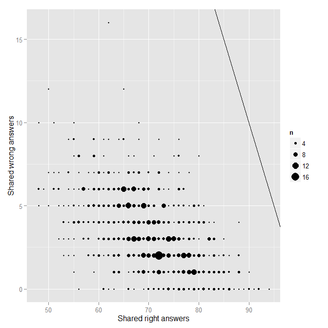
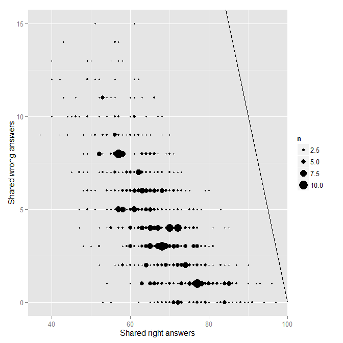
So for each pair of students, we have the number of answers they shared, the number they shared and got correct, and the number they shared and got incorrect. The next step is to plot the number of shared incorrect (wrong) as a function of the number of shared correct (right).
  # Plotting Shared Wrong answers as a function of Shared Right answers
    # Visually inspect for outliers
library(ggplot2)
g0 <- (
ggplot(mydfA, aes(x=rightA, y=wrongA))
	# + geom_point()
	+ stat_sum(aes(size=..n..))
	# + scale_size_area()
	+ geom_abline(intercept=length(answersA), slope=-1)
	+ labs(
		x = "Shared right answers"
		, y = "Shared wrong answers"
	)
	# + stat_smooth()
)
print(g0)
And the resulting image:
Each point on the plot represents a single pair of students. The solid black line indicates the line of “perfect matching.” No one is really near that line at all, which is good. Nonetheless, there is one obvious outlier from the rest of the distribution. Who is that pair of students near the top? You guessed it, it is FC and TS.
head(mydfA[order(mydfA$wrong, decreasing=T),])
    SID1 SID2 shared right wrong Name1 Name2
568   19   20     78    62    16    TS    FC
204    6   20     62    50    12    S6    FC
698   25   39     77    65    12   S25   S39
188    5   39     78    68    10    S5   S39
207    6   23     61    51    10    S6   S23
214    6   30     58    48    10    S6   S30
This is pretty much where Jonathan’s work on this topic stops. In thinking more about this topic though, it occurred to me that we would like some metric to quantify the degree to which the response patterns between a pair of students is an outlier (besides the visual inspection above). The simplest metric is of course the total number shared. Exams that are identical are more likely to reflect cheating. However, shared correct answers are less indicative of cheating than share incorrect answers (assuming students are actually trying to answer correctly). An alternative metric of interest is the number of shared incorrect answers given the total number of answers shared. (You can think of this as similar to a proportion. What proportion of shared answers were incorrect?) In a regression framework, we simply predict the total number of shared incorrect answers from the total number of shared answers. The pairs with large residuals indicate outliers (i.e., potential cheating pairs).
modA <- lm(wrongA ~ sharedA, data=mydfA)
sort(resid(modA)) # Sorting the residuals
op <- par(mfrow=c(2,2))
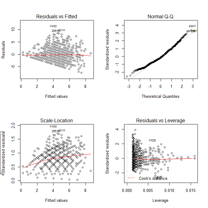
plot(modA) # Looking for outliers
hist(resid(modA), col='cyan') # Plotting the residuals
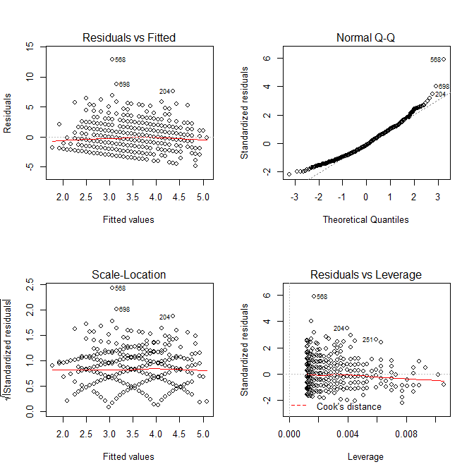
We can take advantage of the diagnostic plots provided by the plot() function to look for outliers. Note that case 568 (our case in question) is quite far from the rest of the data with a residual value of 12.94.
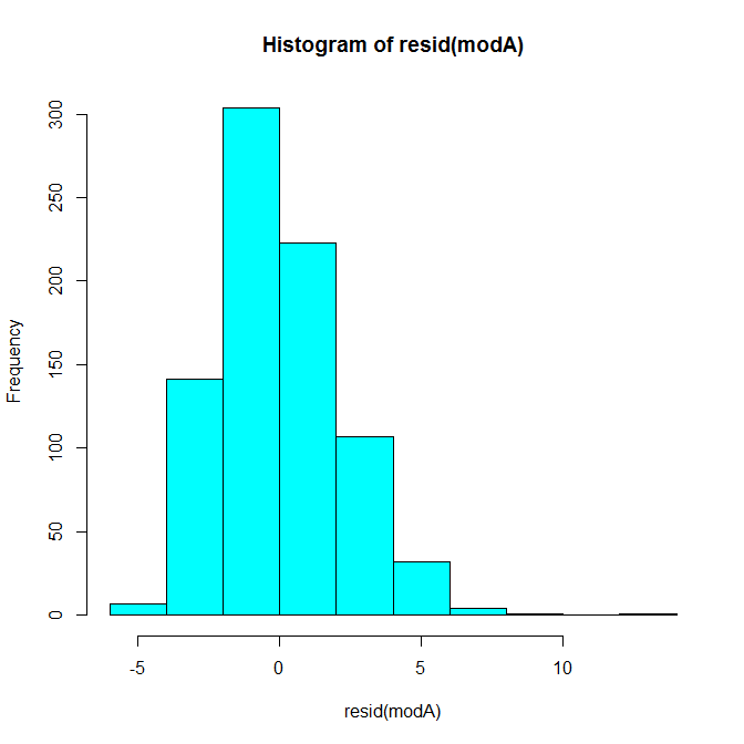
A histogram of the residuals looks like this:
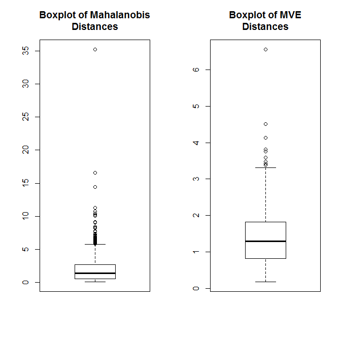
Our case in question is pretty extreme compared to the rest of the distribution. We can also use multivariate outlier detection methods to quantify the distance of each pair of X, Y points (Shared, Shared Incorrect) from the distribution’s center. The first method below here uses Mahalanobis distance and the second uses a robust outlier detection method based on the minimum volume ellipsoid (MVE). In both cases, our pair is question is clearly quite extreme.
  # A non-robust multivariate outlier detection method
mDA <- mahalanobis(mydfA[,3:4], colMeans(mydfA[,3:4]), cov(mydfA[,3:4]))
which.max(mDA)
sort(mDA)

  # A robust outlier detection method
source("http://dornsife.usc.edu/assets/sites/239/docs/Rallfun-v29.txt")
mveA <- outmve(as.matrix(mydfA[,3:4]))
which.max(mveA$dis)
sort(mveA$dis)
op <- par(mfrow=c(1,2))
boxplot(mDA, main="Boxplot of Mahalanobis\nDistances")
boxplot(mveA$dis, main="Boxplot of MVE\nDistances")
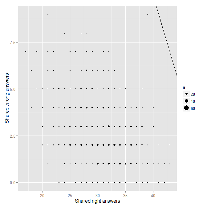
In the .r file linked, these analyses can be replicated for Form B. There is also code for combining the results for both forms into a single chart. Here I will chose show the key graphics for Form B.
Note in the above that no pair of points seems all too extreme. Using the regression approach, the lack of extremity is confirmed with the diagnostic plots:
Ultimately, Form B looks pretty good. Nonetheless, in an effort to be very thorough, I repeated the above analyses for each of the three midterms I gave this past semester. There didn’t appear to be any issues for Midterms 1 and 2. However, one outlier did appear for Midterm 3:
Sure enough, FC was one of the two in the pair. I happen to remember where FC was sitting for the 3rd midterm, but I do not remember where the person with whom FC’s midterm is very similar was sitting that day. I contacted the potential target student to see if he/she could recall, but I have not heard back yet.
Conclusion
What can we conclude here? On one hand, I believe that this provides at least some anecdotal validation for the method described by Jonathan Dushoff in his original post. I physically saw the student cheating and the statistical evidence confirmed my eye-witness account. However, I’m not sure if the statistical evidence alone would be grounds enough for conviction. One problem with the method is that it only identifies pairs of response patterns that look too similar. The statistics alone cannot tell you how those response patterns got similar. The obvious possibility is one student copying off of another, as we have here. However, other possibilities include (a) students working collaboratively on the exam, (b) students who study together or use the same study guide, and (c) randomness. Regarding (c), with any distribution there are bound to be extreme scores. Determining what scores are so extreme as to make randomness a remote possibility would require substantially more work. In this regard, it should be kept in mind that students who perform poorly often share incorrect answers when questions have a single strong distractor option. Regarding (b), it would be interesting to gather data from students to include indicators of studying partners / groups and using shared study guides. We can empirically investigate the question of: do people who study together have more similar exam responses than those who not? Finally, without either a confession or other physical evidence (e.g., an eye-witness, an impossibility based on the seating arrangement), the statistical evidence cannot tell you who in the pair was doing the cheating. Nonetheless, I still believe that using these sorts of tools after the fact may alert professors to the likely frequency of cheating on their exams. And at a bare minimum, the fact that professors can identify potential cheaters based on response patterns alone ought to strike fear in the hearts of those who can peek without getting caught.

Thanks for your kind words. This system seems to be a nice screening tool.
It’s a shame that people cheat and make us worry about them. I hope talking more about it will have some deterrent effect.
I did this once using the g_2 measure described by Frary, R. B., Tideman, T. N., & Watts, T. M. (1977). Indices of cheating on multiple-choice tests. Journal of Educational and Behavioral Statistics, 2(4), 235-256. The nice thing about the measure is that it is N(0,1) under H_0, so if you like that kind of stuff, you can compute a p-value.
I just now looked the article up in Google Scholar, and it looks like there has been a reasonable amount of work since then.
If I get a chance, I’ll edit out identifying information, and send you the report I wrote. I
Thanks Mike. That looks pretty cool and I would appreciate seeing your report!
It must be the end of the semester…
I found the original blog and found the link you provided there to this site. I didn’t really want to waste my time looking at this for my classes, but figured it would be a good chance to get into R a little bit more.
Anyhow, I have one online course where I was suspicious of some cheating. The students are taking the test on their honor not to work together. I thought probably a good majority of students are honorable, and I think that’s still the case. But I had a good number of student falling on the perfect match line for the first exam I’ve looked at. Not cool! When I dug into other aspects of their tests, my worries were confirmed (they took the exam at the same time and even had the same wrong choice on the wrong answer). I’ll be presenting this to my chair or dean to see what they want to do with it.
In my other large class that meets in person and has well proctor exams I only saw one problem on the one exam I checked (and I had been suspicious of this student from before – he failed anyway so I’m not too concerned).
Thanks for posting your more detailed analysis. I have not tried it yet, but I may have to if I need to convince people more rigorously of the problem.